Learning-Based对象敏感指针分析策略

1.Introduction

作者提出了一种partial context-sensitive pointer analysis算法。artifact地址。

motivating example

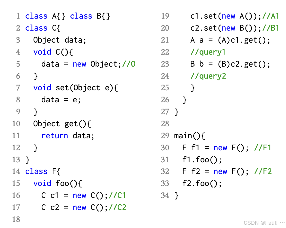
这幅图中在对21行 A a = (A)c1.get(); 和 23行 B b = (B)c2.get(); 进行类型验证 (cast 是否会发生异常) 时需要准确分析出 a 指向object A1，b 指向object B1。如果用context-insensitive方法分析，那么 C::set 方法中 data = e 可推导出 this.data 指向 {A1, B1}，因此 a, b 都会指向 {A1, B1}，会判定 cast 操作不安全。

通过context(object)-sensitive分析可以得出在context C1 下调用 C::set, this.data 指向 A1，在context C2 下调用指向 B1。但是如果全量context-sensitive分析 F1, F2 两个object之后也会展开，而并没有带来精度提升。因此需要一种选择性的context-sensitive策略。

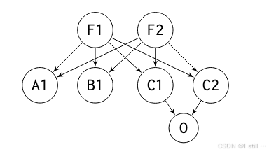
之前的工作${}^{[2],[3]}$提出了object-allocation-graph (上述代码的OAG如下所示) 来描述object之间的context关系。前面示例的OAG如下图所示，F1, F2 的成员函数中分配了 A1, B1, C1, C2。而 C1, C2 的成员函数分配了 O。

下图为policy推导出的选中进行context-sensitive分析的结点满足的条件：

• 1.其所有前驱结点入变边数量在 $[0,\infty ]$，出边数量在 $[2,\infty ]$。

• 2.其所有结点入变边数量在 $[0,\infty ]$，出边数量在 $[0,\infty ]$。

• 3.其所有后继结点入变边数量在 $[2,\infty ]$，出边数量在 $[0,\infty ]$。

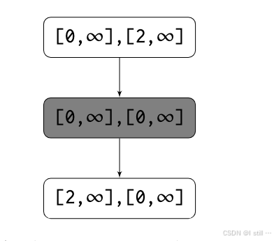
满足条件的object只有 C1, C2。因此对 C1, C2 所有成员函数调用进行context-sensitive分析。

2.Preliminaries

2.1.Baseline Pointer Analysis

Notation	含义	示例
$\mathbb{V}$	程序变量集合	A a 定义了一个 A 类型变量 a
$\mathbb{H}$	堆分配点（allcation site）集合	v = new C 新建了一个 C 类型的堆对象
$\mathbb{M}$	方法（method）集合	void main() { ... } 为 main 方法
$\mathbb{C}$	调用context	定义为一个allocation sites序列
$\mathbb{HC}$	堆context	定义为一个allocation sites序列，和 $\mathbb{HC}$ 等价
$thi{s}_m$	方法 $m$ 的 this 变量
$para{m}_m$	方法 $m$ 的形参
$retur{n}_m$	方法 $m$ 的返回值
$\Vert$（原文的符号打不出来）	在一个序列后append一个元素，用来在context中添加一个allocation site	$s=<a_1,...,a_n>$, $s\Vert a^{{}^{\prime }}=<a_1,...,a_n,a^{{}^{\prime }}>$
$\lceil {\rceil }_k$	取序列后 $k$ 个元素	$\lceil ⟨a_1,a_2,...,a_n⟩{\rceil }_k=⟨a_{n-k+1},...,a_n⟩$

在对象敏感分析中，调用context和堆context等价。

指令类型	示例	关键信息	说明
Alloca	$v=newC$	$(var,heap,inMeth)$	变量(v), 堆对象(new C), 语句所处方法
Copy	$x=y$	$(to,from,inMeth)$	from变量 y, to变量 x, 语句所处方法
Field Load	$x=y.f$	$(to,from,fld,inMeth)$	from变量 y, to变量 x, 加载的fld f, 语句所处方法
Field Store	$x.f=y$	$(to,fld,from,inMeth)$	from变量 y, to变量 x, 写入的fld f, 语句所处方法
Call	$x=y.m_{callee}(arg)$	$(return,base,callee,arg,caller)$	return变量 x，base变量 y，callee函数 m，参数 arg，以及语句所处方法caller

分析输出	映射关系	说明
VarPtsTo	$\mathbb{V}\times \mathbb{C}\to (\mathbb{H}\times \mathbb{HC})$	将变量 $v$ 映射到在context $c$ 下所有所有指向的 (heap context, heap object) 对。
FldPtsTo	$\mathbb{H}\times \mathbb{HC}\times \mathbb{F}\to (\mathbb{H}\times \mathbb{HC})$	将heap object $h$ 的field $f$ ($h.f$) 映射到在context $hc$ 下的所有 (heap context, heap object) 对。
MethodCtx	$\mathbb{M}\to \mathbb{C}$	将method $m$ 映射到所有涉及到的context下

context-sensitive指针分析transfer rule如下，context-insensitive规则本质上就是将所有 $hctx$ 固定为常量。

指令	规则
Alloca	$\frac{(var,heap,inMeth)\in Allocctx\in MethodCtx(inMeth)hctx=\lceil ctx{\rceil }_{maxH}}{(heap,hctx)\in VarPtsTo(var,ctx)}$
Copy	$\frac{(to,from,inMeth)\in Copyctx\in MethodCtx(inMeth)}{VarPtsTo(from,ctx)\subseteq VarPtsTo(to,ctx)}$
Field Load	$\frac{(to,from,fld,inMeth)\in FldLoadctx\in MethodCtx(inMeth)(heap,hctx)\in VarPtsTo(from,ctx)}{FldPtsTo(heap,hctx,fld)\subseteq VarPtsTo(to,ctx)}$
Field Store	$\frac{(to,fld,from,inMeth)\in FldStorectx\in MethodCtx(inMeth)(heap,hctx)\in VarPtsTo(to,ctx)}{VarPtsTo(from,ctx)\in FldPtsTo(heap,hctx,fld)}$
Call	$\frac{(return,base,callee,arg,caller)\in Callctx\in MethodCtx(caller)(heap,hctx)\in VarPtsTo(base,ctx)ct{x}^{{}^{\prime }}=\lceil hctx\Vert heap{\rceil }_{maxK}}{ct{x}^{{}^{\prime }}\in MethodCtx(callee)VarPtsTo(arg,ctx)\subseteq VarPtsTo(para{m}_{callee},ct{x}^{{}^{\prime }})(heap,hctx)\in VarPtsTo(thi{s}_{callee},ct{x}^{{}^{\prime }})VarPtsTo(retur{n}_{callee},ct{x}^{\prime })\subseteq VarPtsTo(return,ctx)}$

2.2.Parameterization

Parametric Object Sensitivity: 前面分析规则中对context深度的处理涉及到计算 $maxK$ 值。作者定义了一个 $ContextAbstraction:H\to [0,maxK]$ 函数将heap object映射到context深度。

Parametric Heap Abstraction: 堆抽象有2种方式， allocation-based以及type-based。allocation-based为每一个 new 调用点分配一个object，type-based为每个class type分配一个object。分析出来的 VarPtsTo 和 FldPtsTo 集合会调整如下，作者定义了一个 $HeapAbstraction$ 函数，如果 $HeapAbstraction(heap)==alloc$，那么object为allocation-site，反之，为 $typeof(heap)$。

• VarPtsTo : $\mathbb{V}\times \mathbb{C}\to ((\mathbb{H}+\mathbb{T})\times \mathbb{HC})$

• FldPtsTo : $(\mathbb{H}+\mathbb{T})\times \mathbb{HC}\times \mathbb{F}\to ((\mathbb{H}+\mathbb{T})\times \mathbb{HC})$

3.Graphick

graphick的策略由feature描述，feature为一个 $(prev,([a,b],[c,d]),succ)$ 3元组。interval pair $([a,b],[c,d])$ 表示被选中的node入边数量在 $[a,b]$ 之间出边数量在 $[c,d]$ 之间。$prev$ 和 $succ$ 为interval序列，描述前驱和后继结点入边和出边数量。

策略由一组参数 $\prod =<F_1,F_2,...F_k>$ 组成，$F_i$ 包含一组feature。策略会给OAG上每一个结点赋予一个degree $j$，如果被 $F_1$ 选中，那么 $j=1$，被 $F_k$ 选中，那么 $j=k$。如果同时被多个feature选中，那么取最大值。degree $j$ 表示进行 j-context-sensitive分析。作者的insight大概在于OAG上不同pattern（比如自身入度多少，出度多少；前驱后继入度、出度）的node应该用不同的上下文敏感度进行分析。具体多少无法人工指定需要学习。策略的学习需要训练样本（也就是几个程序），学习的核心包含一个Learning Minimal Abstraction函数和一个Learning a Set of Features函数。

(1).Learning Minimal Abstraction

指针分析的目标是能够尽可能以最少的代价验证程序中的 cast 操作是否会fail。文中有一个公式 $proved(F_P(a))=proved(F_P(k))$，左边表示基于策略对每个OAG结点赋予的degree进行敏感性分析能够达到的精度（能够验证may-cast-fail的数量），右边表示用精度最高的敏感性分析（每个OAG结点都采用最大值 $k$-context-sensitive分析）。学习的目标就是学到minimal abstraction来分配degree。算法如下，概括一下就是一个搜索算法，复杂度为 $k\cdot 2^{|C_P|}$。$|C_P|$ 可以理解是OAG的结点数量。

(2).Learn a Set of Feature

给每个degree $j$ 学习一组feature $F_j$。过程如下面Algo3所描述。

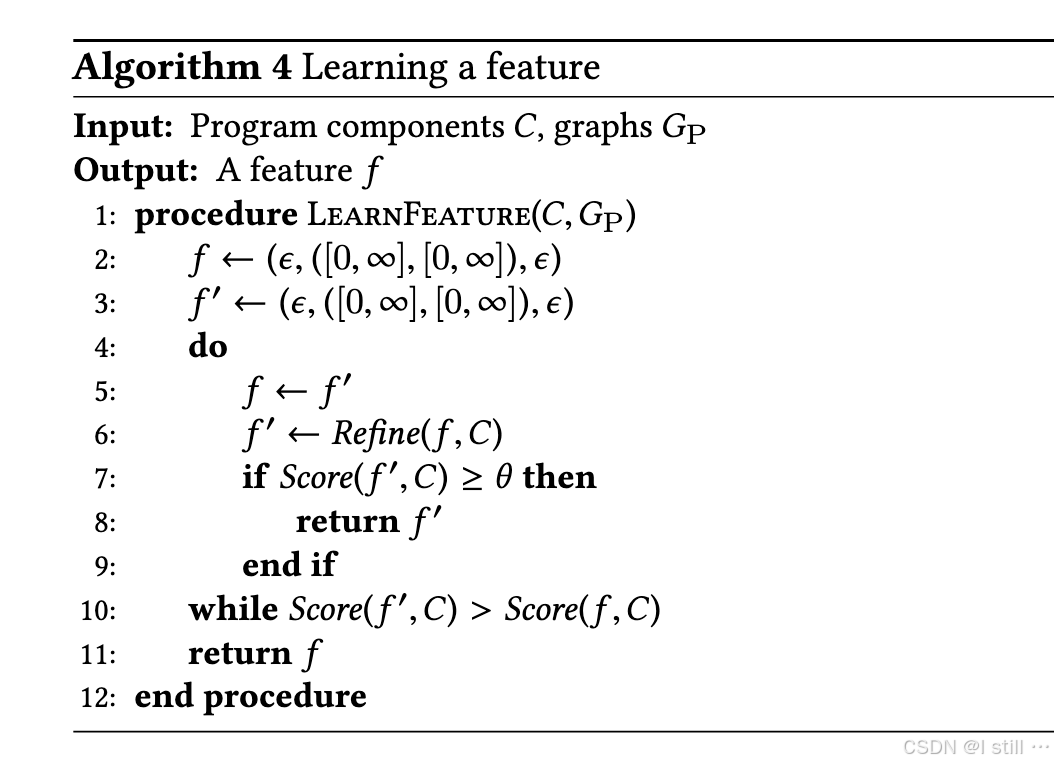
学习单个feature过程如Algo4描述，其中 $Score(f,C)=\frac{\sum \text{P}\in P|C\cap {\gamma }_{G_P}(P)(f)|}{\sum \text{P}\in P|{\gamma }_{G_P}(P)(f)|}$，大概意思是如果策略选中的node都在 $C$ 中，那么score为1；当开始选中 $C$ 之外的node，score开始下降。这里需要人工指定一个阈值 $\theta$。具体过程太复杂了，就不展开了。

4.Evaluation

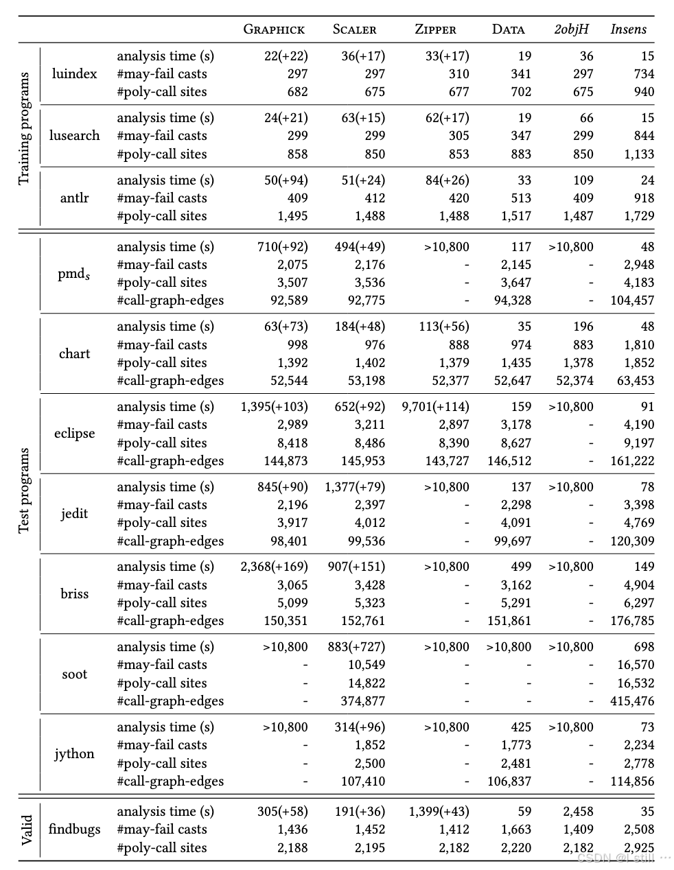
• RQ1: Graphick与baseline策略比较性能如何？

• RQ2: learning开销如何？超参数 $\theta$ 对Graphick性能有什么影响？

• RQ3: 学习到的策略能看出什么insight？

作者基于Doop实现Graphick。对于精度：

• 1.cast-fail分析，作者跟随之前的work采用may-fail分析，也就是只要存在fail的可能就报错。

• 2.作者拿polymorphic call sites和call-edges的数量作为额外精度指标，理论上数量越少精度越高。

每次分析作者设定超时时间3 hours，对于 $\theta$，作者从0.1到0.9每个0.1取值（总共9个）。对于每个feature，作者限定最多选择3 node。

对于benchmark，作者从decapo选择10个(luindex, lusearch, antlr, pmdm , chart, eclipse, fop, bloat, xalan, and jython)，以及从之前工作选择7个 (pmds , jedit, briss, soot, findbugs, JPC, checkstyle)。

这里先放出RQ1的部分结果。RQ2的跳过。

baseline:

• Scaler: 基于OAG的人工制定的object-sensitivity策略。

• Zipper: 基于PFG的人工制定的object-sensitivity策略。

• Data：一种learning-based object-sensitivity策略。

• 2objH: 2-object-sensitivity、1-context sensitivity heap。默认精度上限，开销最大。

• Insens: 不敏感的分析，精度下限，开销最小。

作者选择3个程序作为训练集，1个验证集，剩下13个测试集。效果如下：

RQ3: 作者限制最大上下文敏感度是2，学习的策略总共包含了197个feature，总共包含68个2-object-sensitivity feature，29个2-type-sensitivity feature, 以及100个1-type-sensitivity feature。下图列出了几个top-5 feature，portion表示它们选择的precision-critical nodes的占比，score表示得分。

参考文献

[1].Minseok Jeon, Myungho Lee, and Hakjoo Oh. 2020. Learning graph-based heuristics for pointer analysis without handcrafting application-specific features. Proc. ACM Program. Lang. 4, OOPSLA, Article 179 (November 2020), 30 pages.

[2].Yue Li, Tian Tan, Anders Mùller, and Yannis Smaragdakis. 2018b. Scalability-first Pointer Analysis with Self-tuning Context-sensitivity. In Proceedings of the 2018 26th ACM Joint Meeting on European Software Engineering Conference and Symposium on the Foundations of Software Engineering (Lake Buena Vista, FL, USA) (ESEC/FSE 2018). ACM, New York, NY, USA, 129-140.

[3].Tian Tan, Yue Li, and Jingling Xue. 2016. Making k-Object-Sensitive Pointer Analysis More Precise with Still k-Limiting. In Static Analysis, Xavier Rival (Ed.). Springer Berlin Heidelberg, Berlin, Heidelberg, 489-510.