pandas库数据处理（索引、排序、基本功能）

本文为小编阅读《利用python进行数据分析》第五章的学习笔记。
前面的博客已经介绍了pandas库基本操作、索引等，接下来我们来介绍一下Series和DataFrame中数据交互的基础机制，按照书中的说法，我们只着重于最重要的特性，而不是将所有的特性都给读者一一罗列出来。除了第一个代码之外，其他的代码我们默认库已经完成导入。
(一).重建索引：

1.Series类型的索引重建：输入一个基本的Series类型

import pandas as pd
import numpy as n
a = pd.Series([1, 2, 3, 4, 5], index = ['a', 'b', 'c', 'd', 'e'])
print(a)

输出结果如下：

a    1
b    2
c    3
d    4
e    5
dtype: int64

Process finished with exit code 0

1.1重建索引的代码：使用reindex(方法即可，如果重建的索引数目大于原来元素个数时，python会使用NaN进行自动填充

a = a.reindex(['a', 'b', 'c', 'd', 'e', 'f'])

输出如下：

a    1.0
b    2.0
c    3.0
d    4.0
e    5.0
f    NaN
dtype: float64

注意：重建索引前后的元素类型发生了变化，由 int64 变成了 float64。
2.DataFrame类型重建：我们知道DataFrame类型存在两个索引（index和colums），那么我们可以想见，我们可以将某一个索引进行重建，也应该有一个方法将两个索引全部重建，代码如下：

#我们默认库已经完成导入
a = pd.DataFrame(np.arange(9).reshape((3, 3)), index = ['a', 'b', 'c'], columns = ['one', 'two', 'three'])
print(a)

输出如下：

   one  two  three
a    0    1      2
b    3    4      5
c    6    7      8

Process finished with exit code 0

2.1我们可以只重建行索引（列索引同理），需要注意的一点是，如果我们进行索引重建的时候不给予参数的话，默认重建的是index索引。代码如下：

a = a.reindex(['a', 'b', 'c', 'd'])

结果为

   one  two  three
a  0.0  1.0    2.0
b  3.0  4.0    5.0
c  6.0  7.0    8.0
d  NaN  NaN    NaN

Process finished with exit code 0

2.2我们重建列索引的时候多加了一列，但是该列没有数据，因此python就会自动进行填充

a = a.reindex(index = [1, 2, 3], columns = ['first', 'second', 'third'])

结果为：

   first  second  third
1    NaN     NaN    NaN
2    NaN     NaN    NaN
3    NaN     NaN    NaN

Process finished with exit code 0

我们会发现原来的数据均被替换掉。
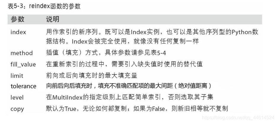
reindex方法的参数：

（二）轴向上删除条目：我们使用drop()方法来删除一个含有指示值或轴向上的删除值的新对象。
1.对Series类型数据集的删除，首先我们创建一个Series类型的数据集。

a = pd.Series(np.arange(3), index = ['a', 'b', 'c'])
print(a)

输出如下：

a    0
b    1
c    2
dtype: int32

Process finished with exit code 0

1.1删除操作代码为：

a = a.drop('a', axis = 'index')

删除后的结果为：

b    1
c    2
dtype: int32

Process finished with exit code 0

2.对DataFrame类型数据集的删除操作：先进行基础数据集的创建。

a = pd.DataFrame(np.arange(9).reshape((3, 3)), index = ['a', 'b', 'c'], columns = ['one', 'two', 'three'])
print(a)

输出为：

   one  two  three
a    0    1      2
b    3    4      5
c    6    7      8

Process finished with exit code 0

2.1删除行数据（对Index进行操作）：与Series类型的区别是，在进行DataFrame类型数据集数据的删除的时候，我们要在drop中加上一个参数 axis,如果删除的是行索引，就令axis = ‘index’，对于列索引同理。

a = a.drop('a', axis = 'index')

删除后的数据集为：

   one  two  three
b    3    4      5
c    6    7      8

Process finished with exit code 0

我们可以发现原先行索引的 a 这一行的数据已经消失。同理我们也可以对列索引进行删除
（三）索引：

1.Series类型的索引：该类型索引与NumPy数组索引功能类似，只不过Series的索引值不仅仅局限于整数，它可以是index的值，区间等。首先我们还是首先创建Series类型数据。

a = pd.Series(np.arange(4.), index = ['a', 'b', 'c', 'd'])
print(a)

输出为：

a    0.0
b    1.0
c    2.0
d    3.0
dtype: float64

Process finished with exit code 0

1.1我们直接使用Index 的名称进行索引

1.2我们也可以使用类似于切片的方式来进行取出索引对应的元素。注意：这里的切片的区间两边均为闭区间，与python列表的切片有区别。

1.3或者我们直接使用索引来进行对应元素的输出。注意：采用对应索引进行输出的时候，索引的输入方式。

print(a[['a', 'c']])

输出结果为：

a    0.0
c    2.0
dtype: float64

Process finished with exit code 0

2.DataFrame类型数据的索引：首先还是进行数据集的建立：

a = pd.DataFrame(np.arange(16).reshape(4, 4), index = ['a', 'b', 'c', 'd'],
                 columns = ['one', 'two', 'three', 'four'])
print(a)

输出为：

   one  two  three  four
a    0    1      2     3
b    4    5      6     7
c    8    9     10    11
d   12   13     14    15

Process finished with exit code 0

2.1我们可以使用列索引（行索引）来将某一列（行）的所有元素进行输出（结果会自动带上行（列）索引）

print(a['two'])

输出为：

a     1
b     5
c     9
d    13
Name: two, dtype: int32

Process finished with exit code 0

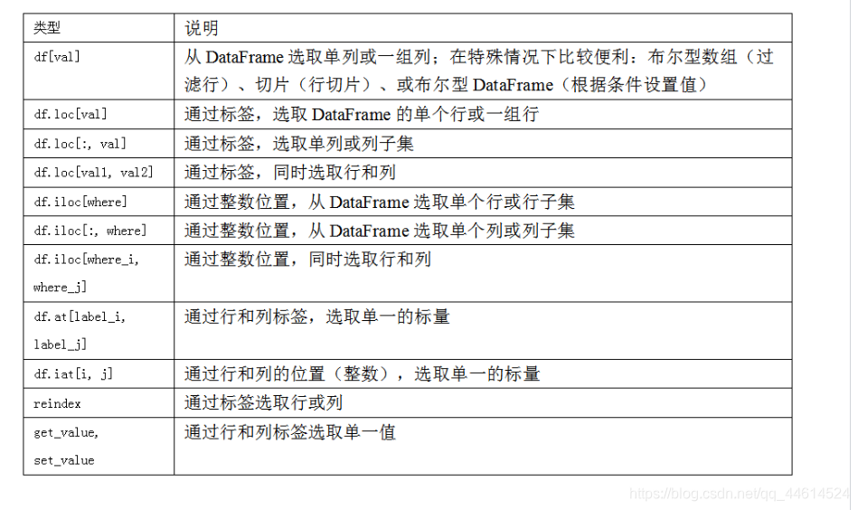
3.针对DataFrame类型在行上的标签索引，小编介绍一下loc()和 iloc()，他们允许用户使用轴标签（loc)整数标签 (iloc)，使用风格与我们在NumPy中的索引方式类似。我们简单的创建一个数据集：（当我们自定义标签之后，我们能够体现出轴标签与整数标签的差距了）轴标签就是使用Index，而整数标签就会像数组那样。

a = pd.DataFrame(np.arange(12).reshape(3, 4))
print(a)

创建的结果如下：

   0  1   2   3
0  0  1   2   3
1  4  5   6   7
2  8  9  10  11

Process finished with exit code 0

我们使用对应的索引来进行数据的选取。（下标的标记类似数组，从0开始）


（四）Dataframe与Series之间的算术操作：

1.Dataframe算术操作：首先进行数据集的创建：

a = np.arange(12).reshape(3, 4)
print(a)

数据集的输出为：

[[ 0  1  2  3]
 [ 4  5  6  7]
 [ 8  9 10 11]]

Process finished with exit code 0

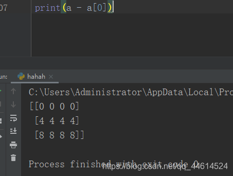
我们先看一下，数据元素（a[0]）的输出

print(a[0])

接下来我们进行算术运算，如下图，图中我们可以看到：当我们用整个数据集去减第一行的数据的时候，减法在每一行都进行了操作，这就是我们所谓的广播机制。

对于Series，也有类似的操作：首先我们进行数据集的创建：

a = pd.DataFrame(np.arange(12).reshape(3, 4), index = ['a', 'b', 'c'], columns = ['one', 'two', 'three', 'four'])
print(a)

创建好的数据集如下：

   one  two  three  four
a    0    1      2     3
b    4    5      6     7
c    8    9     10    11

Process finished with exit code 0

我们模仿DataFrame的算术方法来进行广播计算（个人的叫法，未必正确）。注意：这里的DataFrame类型的索引与Series有区别，我们要使用.iloc()方法进行索引。

a = pd.DataFrame(np.arange(12).reshape(3, 4), index = ['a', 'b', 'c'], columns = ['one', 'two', 'three', 'four'])
b = a.iloc[0]
print(a - b)

输出的结果如下：我们可以看出这与我们预想的（与Series）结果一样，同样进行了广播运算。

   one  two  three  four
a    0    0      0     0
b    4    4      4     4
c    8    8      8     8

Process finished with exit code 0

(五) 排序：
1.Series类型：首先我们创建一个Series数据集：

a = pd.Series([1, 3, 4, 2], index = ['a', 'c', 'd', 'b'])

输出为：

a    1
c    3
d    4
b    2
dtype: int64

Process finished with exit code 0

1.1 我们可以看到Index的顺序是打乱排列的。我们可以采用如下代码进行索引的排序：

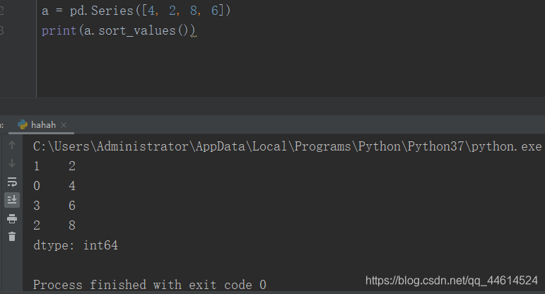
a.sort_values()

索引排好序的结果为：

a    1
b    2
c    3
d    4
dtype: int64

Process finished with exit code 0

我们可以看到现在的行索引已经完成排序，列排序同理。
2.2 我们也可以对Series的值进行排序：（如果有缺失值的话，缺失值会被放到最后面）

2.DataFrame类型：首先我们生成数组

a = pd.DataFrame(np.array([1, 3, 4, 2, 6, 5, 7, 0, 8]).reshape(3, 3), index = ['a', 'c', 'b'],
                 columns = ['one', 'three', 'two'])

生成的数据集为：

   one  three  two
a    1      3    4
c    2      6    5
b    7      0    8

Process finished with exit code 0

2.1 对行索引进行排序的结果为：

   one  three  two
a    1      3    4
b    7      0    8
c    2      6    5

Process finished with exit code 0

我们可以看到行索引已经完成排序。（默认升序排列）