机器学习—降维算法1LDA线性判别分析(实战)

代码1，一步一步去操作LDA

代码2，直接从sklearn调用LDA方法，指定降维

 

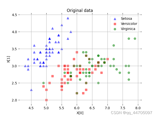
原始数据展示结果

 

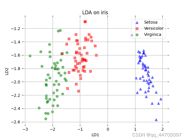
特征数据降维后展示结果

import pandas as pd
import numpy as np
from matplotlib import pyplot as plt
from sklearn.preprocessing import LabelEncoder
# 自己来定义列名
feature_dict = {i:label for i,label in zip(range(4),('sepal length in cm','sepal width in cm','petal length in cm','petal width in cm', ))}  #四个特征

label_dict = {i:label for i,label in zip(range(1,4),('Setosa','Versicolor','Virginica'))}   #三个标签

# 数据读取，大家也可以先下载下来直接读取
df = pd.io.parsers.read_csv(
    filepath_or_buffer='https://archive.ics.uci.edu/ml/machine-learning-databases/iris/iris.data',
    header=None,
    sep=',',
    )
# 指定列名
df.columns = [l for i,l in sorted(feature_dict.items())] + ['class label']

#print(df.head())



#获取数据
X = df[['sepal length in cm','sepal width in cm','petal length in cm','petal width in cm']].values # 特征数据
y = df['class label'].values  #标签

# 使用sklearn中的LabelEncoder()用于快速完成标签的转换，先fit再transform
# 制作标签{1: 'Setosa', 2: 'Versicolor', 3:'Virginica'}
enc = LabelEncoder()# LabelEncoder 是对不连续的数字或者文本进行编号（连续的会是同一个编号）
label_encoder = enc.fit(y)
y = label_encoder.transform(y) + 1  # 将标签转换成1,2,3，
#
#

#设置小数点的位数
np.set_printoptions(precision=4)
#这里会保存所有的均值（数据的中心点位置）
mean_vectors = []
# 要计算3个类别各个特征值 的均值
for cl in range(1,4):
    # 求当前类别各个特征均值
    mean_vectors.append(np.mean(X[y==cl], axis=0))
    print('均值类别 %s: %s\n' %(cl, mean_vectors[cl-1]))


 #计算类内的散布均值
# 原始数据中有4个特征
S_W = np.zeros((4,4))
# 要考虑不同类别，自己算自己的
for cl,mv in zip(range(1,4), mean_vectors):

    class_sc_mat = np.zeros((4,4))
    # 选中属于当前类别的数据
    for row in X[y == cl]:
        # 这里相当于对各个特征分别进行计算，用矩阵的形式
        row, mv = row.reshape(4,1), mv.reshape(4,1)
        # 跟公式一样
        class_sc_mat += (row-mv).dot((row-mv).T)
        #print( class_sc_mat)
    S_W += class_sc_mat

print('类内散布矩阵:\n', S_W)

# 全局均值
overall_mean = np.mean(X, axis=0)
print(overall_mean )
# 构建类间散布矩阵
S_B = np.zeros((4,4))
# 对各个类别进行计算
for i,mean_vec in enumerate(mean_vectors):
    #当前类别的样本数
    n = X[y==i+1,:].shape[0]
    mean_vec = mean_vec.reshape(4,1)
    print(mean_vec)
    overall_mean = overall_mean.reshape(4,1)
    # 如上述公式进行计算
    S_B += n * (mean_vec - overall_mean).dot((mean_vec - overall_mean).T)
    print(S_B)

print('类间散布矩阵:\n', S_B)
#
# #求解矩阵特征值，特征向量np.linalg.eig()是numpy求矩阵的特征值与特征向量
eig_vals, eig_vecs = np.linalg.eig(np.linalg.inv(S_W).dot(S_B)) # np.linalg.inv()求矩阵的逆
# 拿到每一个特征值和其所对应的特征向量
for i in range(len(eig_vals)):
    eigvec_sc = eig_vecs[:,i].reshape(4,1)
    print('\n特征向量 {}: \n{}'.format(i+1, eigvec_sc.real))
    print('特征值 {:}: {:.2e}'.format(i+1, eig_vals[i].real))
#
#
#特征值和特征向量配对
eig_pairs = [(np.abs(eig_vals[i]), eig_vecs[:,i]) for i in range(len(eig_vals))]

# 按特征值大小进行排序
eig_pairs = sorted(eig_pairs, key=lambda k: k[0], reverse=True)

print('特征值排序结果:\n')
for i in eig_pairs:
    print(i[0])

print('特征值占总体百分比:\n')
eigv_sum = sum(eig_vals)
for i,j in enumerate(eig_pairs):
    print('特征值 {0:}: {1:.2%}'.format(i+1, (j[0]/eigv_sum).real))

# 选择前两维特征
W = np.hstack((eig_pairs[0][1].reshape(4,1), eig_pairs[1][1].reshape(4,1)))
print('矩阵W:\n', W.real)
#
# #对特征进行降维
X_lda = X.dot(W)
print(X_lda.shape)
#

# 原始数据可视化
from matplotlib import pyplot as plt
# 可视化展示
def plot_step_lda():

    ax = plt.subplot(111)
    for label,marker,color in zip(
        range(1,4),('^', 's', 'o'),('blue', 'red', 'green')):

        plt.scatter(x=X[:,0].real[y == label],
                y=X[:,1].real[y == label],
                marker=marker,
                color=color,
                alpha=0.5,
                label=label_dict[label]
                )

    plt.xlabel('X[0]')
    plt.ylabel('X[1]')

    leg = plt.legend(loc='upper right', fancybox=True)
    leg.get_frame().set_alpha(0.5)
    plt.title('Original data')

    # 把边边角角隐藏起来
    plt.tick_params(axis="both", which="both", bottom="off", top="off",
            labelbottom="on", left="off", right="off", labelleft="on")

    # 为了看的清晰些，尽量简洁
    ax.spines["top"].set_visible(False)
    ax.spines["right"].set_visible(False)
    ax.spines["bottom"].set_visible(False)
    ax.spines["left"].set_visible(False)

    plt.grid()
    plt.tight_layout
    plt.show()

plot_step_lda()
#
#
# #降维后数据展示
from matplotlib import pyplot as plt
# 可视化展示
def plot_step_lda():

    ax = plt.subplot(111)
    for label,marker,color in zip(
        range(1,4),('^', 's', 'o'),('blue', 'red', 'green')):

        plt.scatter(x=X_lda[:,0].real[y == label],
                y=X_lda[:,1].real[y == label],
                marker=marker,
                color=color,
                alpha=0.5,
                label=label_dict[label]
                )

    plt.xlabel('LD1')
    plt.ylabel('LD2')

    leg = plt.legend(loc='upper right', fancybox=True)
    leg.get_frame().set_alpha(0.5)
    plt.title('LDA on iris')

    # 把边边角角隐藏起来
    plt.tick_params(axis="both", which="both", bottom="off", top="off",
            labelbottom="on", left="off", right="off", labelleft="on")

    # 为了看的清晰些，尽量简洁
    ax.spines["top"].set_visible(False)
    ax.spines["right"].set_visible(False)
    ax.spines["bottom"].set_visible(False)
    ax.spines["left"].set_visible(False)

    plt.grid()
    plt.tight_layout
    plt.show()

plot_step_lda()

 import pandas as pd
import numpy as np
from matplotlib import pyplot as plt
from sklearn.preprocessing import LabelEncoder
# 自己来定义列名
feature_dict = {i:label for i,label in zip(range(4),('sepal length in cm','sepal width in cm','petal length in cm','petal width in cm', ))}  #四个特征

label_dict = {i:label for i,label in zip(range(1,4),('Setosa','Versicolor','Virginica'))}   #三个标签

# 数据读取，大家也可以先下载下来直接读取
df = pd.io.parsers.read_csv(
    filepath_or_buffer='https://archive.ics.uci.edu/ml/machine-learning-databases/iris/iris.data',
    header=None,
    sep=',',
    )
# 指定列名
df.columns = [l for i,l in sorted(feature_dict.items())] + ['class label']

#print(df.head())



#获取数据
X = df[['sepal length in cm','sepal width in cm','petal length in cm','petal width in cm']].values # 特征数据
y = df['class label'].values  #标签

# 使用sklearn中的LabelEncoder()用于快速完成标签的转换，先fit再transform
# 制作标签{1: 'Setosa', 2: 'Versicolor', 3:'Virginica'}
enc = LabelEncoder()# LabelEncoder 是对不连续的数字或者文本进行编号（连续的会是同一个编号）
label_encoder = enc.fit(y)
y = label_encoder.transform(y) + 1  # 将标签转换成1,2,3，

# 直接在sklearn 中调用 LinearDiscriminantAnalysis，指定降维后的维数

from sklearn.discriminant_analysis import LinearDiscriminantAnalysis as LDA

# LDA
sklearn_lda = LDA(n_components=2)
X_lda_sklearn = sklearn_lda.fit_transform(X, y)


def plot_scikit_lda(X, title):

    ax = plt.subplot(111)
    for label,marker,color in zip(
        range(1,4),('^', 's', 'o'),('blue', 'red', 'green')):

        plt.scatter(x=X[:,0][y == label],
                    y=X[:,1][y == label] * -1, # flip the figure
                    marker=marker,
                    color=color,
                    alpha=0.5,
                    label=label_dict[label])

    plt.xlabel('LD1')
    plt.ylabel('LD2')

    leg = plt.legend(loc='upper right', fancybox=True)
    leg.get_frame().set_alpha(0.5)
    plt.title(title)

    # hide axis ticks
    plt.tick_params(axis="both", which="both", bottom="off", top="off",
            labelbottom="on", left="off", right="off", labelleft="on")

    # remove axis spines
    ax.spines["top"].set_visible(False)
    ax.spines["right"].set_visible(False)
    ax.spines["bottom"].set_visible(False)
    ax.spines["left"].set_visible(False)

    plt.grid()
    plt.tight_layout
    plt.show()

plot_scikit_lda(X_lda_sklearn, title='Default LDA via scikit-learn')

参考文档：《跟着迪哥学Python数据分析与机器学习实战》