自由曲面面型设计【角谱衍射理论，GS算法】

本文链接：https://blog.csdn.net/qq_44791407/article/details/133125543

本文介绍了解决光波通过自由曲面后相位变化问题的方法，通过GS算法求解自由曲面的面型分布，给出了MATLAB代码示例，包括数据处理、振幅约束和相位优化过程。

摘要生成于 C知道，由 DeepSeek-R1 满血版支持，前往体验 >

1. 背景

在我发布光波传输的角谱理论【理论，实例及matlab代码】这篇文章之后，有很多人对其中的自由曲面厚度矩阵有所需求，但是由于某些原因，该矩阵不能公开。但是，我在评论区也曾说可以通过反向设计的方式得到自由曲面的厚度矩阵，本篇文章就是基于此而撰写的。

2. 问题与解决方案

2.1 问题描述

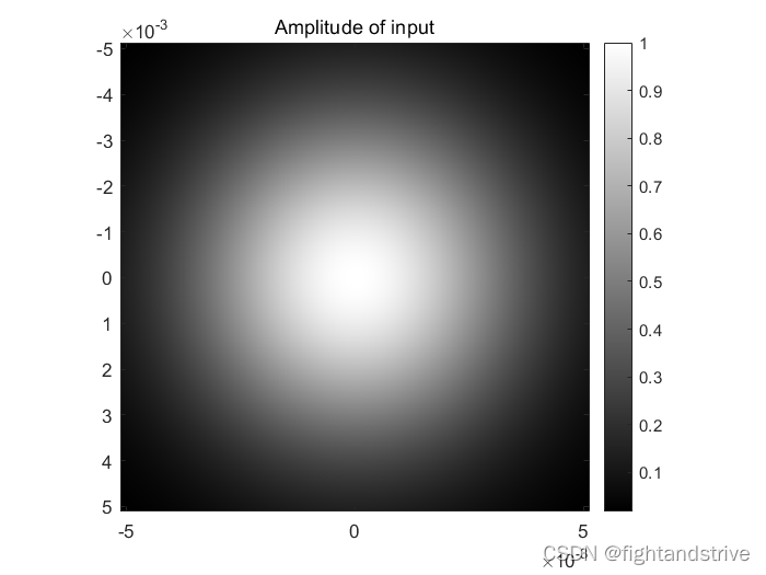
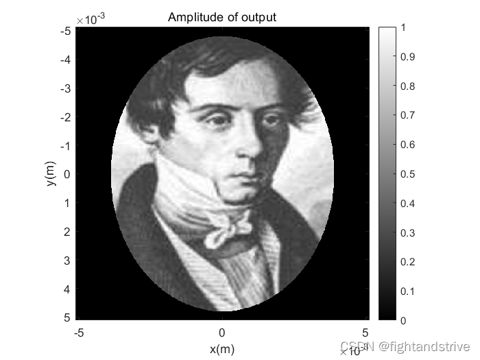
假设采用一个振幅分布为高斯型的平面光源（大小10.24mm*10.24mm，波长532nm，束腰为5.32mm，如图1所示）垂直照射一个自由曲面（最大厚度 $D_{max}$ 为3mm，折射率 $n$ 为1.494），透过自由曲面的光波在自由空间传播200mm后得到一张图2所示的菲涅尔的图像，图像有效区域为一个椭圆区域，长轴为9.6mm，短轴为7.8mm，试求解自由曲面的面型分布函数 $m(x,y)$ 。

2.2 问题分析

对于这个问题，解决的方案其实有很多。首先明确已知条件，是两个振幅图像，而未知条件是自由曲面的面型分布，即光波透过自由曲面之后的相位变化未知。所以，这个问题就变成了一个优化的问题，及找到一个相位信息，使得其满足两个振幅约束条件，这就是一个经典GS算法所面对的问题。

2.3 解决方案

2.3.1 用GS算法求解自由曲面的相位分布

经典的GS算法怎么实现，可以参考GS算法简介这篇文章。GS算法基本流程如图3所示，其基本步骤描述如下：

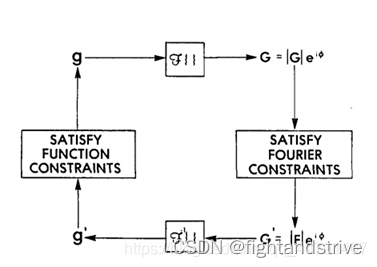
1. 给出输入面的初始复振幅估计；在此问题中，输入面是自由曲面的后表面，故输入振幅为高斯光源 $s(x,y)$ ，初始相位就为自由曲面引入的相位变化 $\phi_0 (x,y)$ ，初始的复振幅分布 $g(x,y)=s(x,y)e^{(j*\phi_0(x,y))}$ ，当然，因为自由曲面的面型，即相位透过率函数是未知的， $\phi_0 (x,y)$ 可以随机取值，全0，全1，或者随机值都可以。
2.通过角谱衍射的方式，将 $g(x,y)$ 传输到200mm处，得到输出面的复振幅分布 $G_k(x,y)=\Im^{-1}[\Im(g_0(x,y))*H(f_x,f_y))]=G(x,y)e^{(j*\Phi(x,y))},$

其中， $H(f_x,f_y)$ 是角谱衍射在自由空间中的传递函数，下标 $k$ 表示当前迭代次数，可以表示为

$H(f_x,f_y)=\textup{exp}(j2\pi z \sqrt{(\frac{1}{\lambda})^2-f_x^2-f_y^2)}$

其中， $z$ 是传输距离， $\lambda$ 是照明光波在真空中的波长。

3. 在输出面内作适当的约束；将输出面的振幅替换为想要得到的振幅，即菲涅尔的图像 $F(x,y)$ ，即 $G'_k(x,y)=F(x,y)e^{(j*\Phi(x,y))}$ ，得到更新后的输出面复振幅。
4. 通过角谱衍射的方式，将 $G'_k(x,y)$ 传输到输入面，得到更新后的输入面复振幅分布

$g'_k(x,y)=f(x,y)e^{(j*\phi_k(x,y))}$ 。

5.在输入面内作适当的约束；将输入面的振幅替换为想要得到的振幅，即高斯照明光 $s(x,y)$ ，得到更新后的输入面复振幅估计

$g_k(x,y)=s(x,y)e^{(j*\phi_k(x,y))}$ 。

6.重复上述的5个步骤，直到满足终止条件时，得到的 $\phi_k(x,y)$ 就是自由曲面的相位分布，条件可以是迭代次数、频域误差、空域误差等。

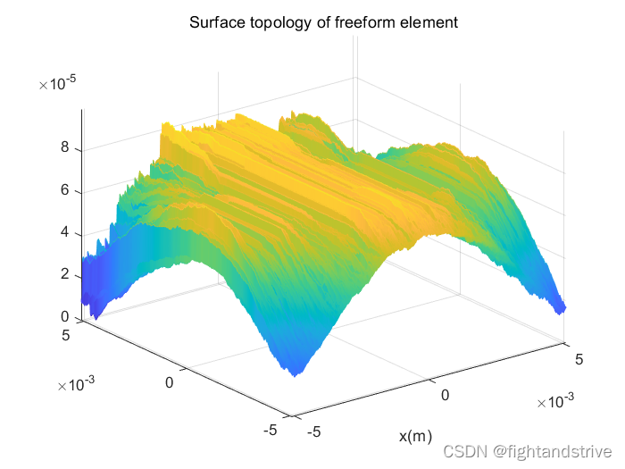
2.3.2 将自由曲面的相位分布转换为面型分布

首先看正向模型，振幅分布为高斯型的平面光源垂直照射一个自由曲面（最大厚度 $D_{max}$ 为3mm，折射率 $n$ 为1.494）后，其相位变换为

$\phi (x,y)=[D_{max}+(n-1)*m(x,y)]*2\pi/ \lambda$

所以，其面型分布就可以表示为

$m(x,y) = [\lambda * \phi (x,y) /2 \pi)- D_{max}] /(n-1)$ 。

3. matlab代码

%%% Copyrights Sep 21, 2023.
clc;
clearvars;
close all;
%% Generate the input Gaussian beam(modulus constraint on input plane)
mm=1e-3;
nm=1e-9;
lambda=532*nm;% wavelength
k=2*pi/lambda;% wavevector
n=1.494;% The rafractive index of freeform elements 
SL=10.24*mm ;% Side length
N=512*1;% samples for side length
dx=SL/N;%sample interval
d=200*mm;% The distance between the input and target planes
x = -0.5*SL:dx:0.5*SL-dx;
y = x;
[X,Y]=meshgrid(x,y);
E_input=exp(-2*((X /(0.5* SL)).^2+(Y/(0.5* SL)).^2)); %The input Gaussian beam
figure;
imagesc(x,y,E_input);
colormap gray;
colorbar;
title('Amplitude of input');
axis square;

%% Generate the output Fresnel with a ellipsed support zone(constraint on output plane)
semi_major = 4.8*mm;
semi_minor = 3.9*mm;
ellipse = ((X.^2/semi_minor.^2+Y.^2/semi_major.^2)<=1);
Fresnel  = imread('Fresnel.jpg');
Fresnel = double(imresize(Fresnel,[512 512]));
Fresnel = Fresnel./max(Fresnel(:));
output_constraint = Fresnel.*ellipse;
figure;
imagesc(x,y,output_constraint);
axis square;
xlabel('x(m)');
ylabel('y(m)');
colormap gray;
colorbar;
title('Amplitude of output');


%% load phase modulataion by the freeform surface as the initial phase guess
P_input  = exp(1i*ones(N,N)); % all zero phase for inital guess
figure;mesh(X,Y,angle(P_input));
title('Initial phase guess');
xlabel('x(m)');
ylabel('y(m)');
zlabel('\phi');
u1 = E_input.*P_input;

%% obtain the output field wiht Fresnel diffraction
fx = -1/(2*dx):1/SL:1/(2*dx)-1/SL;  %freq coords
[FX,FY] = meshgrid(fx,fx);
H = exp(1i*k*d*sqrt(1-(lambda*FX).^2-(lambda*FY).^2));  %trans func
U1 =fftshift(fft2(u1));  %shift.fft source filed
U2 = H.*U1;    %multiply
u2 = ifft2(ifftshift(U2));
figure;
imagesc(x,y,abs(u2));
axis square;
xlabel('x(m)');
ylabel('y(m)');
colormap gray;
colorbar;
title('Initial amplitude of output');

%% refine the phase distribution using GS algorithm
phase_old = P_input;
H_forward=exp(1i*k*d*sqrt(1-(lambda*FX).^2-(lambda*FY).^2));  %trans func
H_inverse=exp(-1i*k*d*sqrt(1-(lambda*FX).^2-(lambda*FY).^2));  %trans func
for count = 1:50
     input = E_input.*phase_old;
     Input = fftshift(fft2(input));  %shift.fft source filed
     Output = H_forward.*Input;    %multiply
     output = ifft2(ifftshift(Output));
     output_update = output_constraint.*output./abs(output);
     Output_update = fftshift(fft2(output_update));
     Input_update = Output_update.*H_inverse;
     input_update = ifft2(ifftshift(Input_update));
     phase_old = input_update./abs(input_update);
end
figure;mesh(X,Y,angle(input_update));
title('Refined phase distribution');
xlabel('x(m)');
ylabel('y(m)');
zlabel('\phi');

figure;
imagesc(x,y,abs(output));
axis square;
xlabel('x(m)');
ylabel('y(m)');
colormap gray;
colorbar;
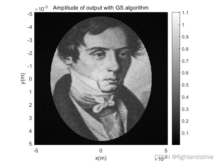
title('Amplitude of output with GS algorithm');

%% transform phase to surface topology
phase = angle(input_update);
phase = unwrap(unwrap(phase,[],2),[],1);
m = (lambda*phase/(2*pi) - 3*mm)/(n-1);
dm = lambda/(n-1); % thickness alter when phase increase 2pi
deltaM = ceil(abs(min(m(:)))/dm); % added minimun thickness for current m
m = m + deltaM*dm;
figure;mesh(X,Y,m);
title('Surface topology of freeform element');
xlabel('x(m)');