python利用pymannkendall包进行Theil-Sen Median斜率估计和Mann-Kendall检验

介绍一下Theil-Sen Median斜率估计和Mann-Kendall趋势分析，这两种方法经常结合使用，前者用于估计趋势的斜率，后者用于检验趋势的显著性。如多年NPP或者NDVI的趋势分析。

Theil-Sen斜率估计

Theil-Sen回归是一种鲁棒线性回归方法，用于减小异常值对拟合结果的影响。与最小二乘法和一些其他回归方法不同，Theil-Sen回归使用了一种称为中位数斜率的统计量来进行参数估计，从而提高回归模型的鲁棒性。

Theil-Sen回归的步骤如下：

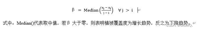
对于给定的自变量和因变量数据，计算所有点对（两两数据点）的斜率。

然后找出所有斜率的中位数，这个中位数就是Theil-Sen回归的估计斜率。

使用估计的斜率，可以计算出拟合的截距。

Theil-Sen回归的优点在于它对于数据中的异常值有很好的鲁棒性。因为它使用的是中位数而不是均值来估计斜率，中位数对于异常值不敏感，能够较好地抵抗异常值的影响。这使得Theil-Sen回归在处理有较多异常值的数据时表现良好。

另外，Theil-Sen回归是一种非参数方法，它不需要对数据的分布进行假设，更加灵活。

Mann-Kendall(MK)检验

Mann-Kendall(MK)检验是一种非参数的时间序列趋势性检验方法，其不需要测量值服从正太分布，不受缺失值和异常值的影响，适用于长时间序列数据的趋势显著检验。其过程如下：对于序列Xt = x1,x2,⋯xn，先确定所有对偶值（ xi , xj , j > i ）中xi与xj的大小关系（设为S）。做如下假设：H0,序列中的数据随机排列，即无显著趋势；H1，序列存在上升或下降趋势。检验统计量S计算公式为（在Z的计算

上式中，当S>0时，分子为S-1
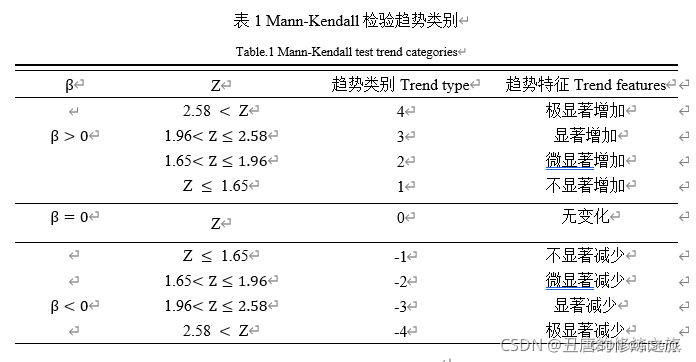
同样采用双边趋势检验，在给定显著性水平下，在正态分布表中查得临界值 Z1－α/2。当|Z|≤Z1－α/2时，接受原假设，即趋势不显著; 若|Z| ＞Z1－α/2，则拒绝原假设，即认为趋势显著。本文给定显著性水平 α = 0.05，则临界值 Z1－α/2 = ±1.96，当Z的绝对值大于1.65、1.96和2.58时，表示趋势分别通过了信度为90%、95%和99%的显著性检验。趋势显著性的判断方法如下：

不过也经常以Z=1.96为界限：

• 显著水平通常为0.05
• Z的绝对值大于1.96为显著
• Z的绝对值小于1.96为不显著

下面介绍如何使用python实现：

使用python进行Theil-Sen Median斜率估计和Mann-Kendall检验主要用到了pymannkendall包，pymannkendall包的安装如下：

用户	安装
Linux	sudo pip install pymannkendall
Windows	pip install pymannkendall
conda	conda install -c conda-forge pymannkendall
others	git clone https://github.com/mmhs013/pymannkendall
克隆存储库	cd pymannkendall python
然后安装	setup.py install

pymannkendall的详细介绍：

https://pypi.org/project/pymannkendall/

import numpy as np
import pymannkendall as mk

# Data generation for analysis
data = np.random.rand(360,1)

result = mk.original_test(data)
print(result)

运行代码后结果：

Mann_Kendall_Test(trend='no trend', h=False, p=0.9507221701045581, z=0.06179991635055463, Tau=0.0021974620860414733, s=142.0, var_s=5205500.0, slope=1.0353584906597959e-05, intercept=0.5232692553379981)

可以指定输出的元素：

print(result.slope)

或者

trend, h, p, z, Tau, s, var_s, slope, intercept = mk.original_test(data)

输出的内容解释：

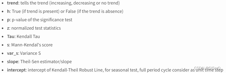
输出包含了Theil-Sen Median斜率估计和Mann-Kendall检验的内容。

也可以自定义函数：

from __future__ import division
import numpy as np
import pandas as pd
from scipy import stats
from scipy.stats import norm

def mk_test(x, alpha=0.05):
    """
    This function is derived from code originally posted by Sat Kumar Tomer
    (satkumartomer@gmail.com)
    See also: http://vsp.pnnl.gov/help/Vsample/Design_Trend_Mann_Kendall.htm
    The purpose of the Mann-Kendall (MK) test (Mann 1945, Kendall 1975, Gilbert
    1987) is to statistically assess if there is a monotonic upward or downward
    trend of the variable of interest over time. A monotonic upward (downward)
    trend means that the variable consistently increases (decreases) through
    time, but the trend may or may not be linear. The MK test can be used in
    place of a parametric linear regression analysis, which can be used to test
    if the slope of the estimated linear regression line is different from
    zero. The regression analysis requires that the residuals from the fitted
    regression line be normally distributed; an assumption not required by the
    MK test, that is, the MK test is a non-parametric (distribution-free) test.
    Hirsch, Slack and Smith (1982, page 107) indicate that the MK test is best
    viewed as an exploratory analysis and is most appropriately used to
    identify stations where changes are significant or of large magnitude and
    to quantify these findings.
    Input:
        x:   a vector of data
        alpha: significance level (0.05 default)
    Output:
        trend: tells the trend (increasing, decreasing or no trend)
        h: True (if trend is present) or False (if trend is absence)
        p: p value of the significance test
        z: normalized test statistics
    Examples
    --------
      >>> x = np.random.rand(100)
      >>> trend,h,p,z = mk_test(x,0.05)
    """
    n = len(x)
    # calculate S
    s = 0
    for k in range(n - 1):
        for j in range(k + 1, n):
            s += np.sign(x[j] - x[k])

    # calculate the unique data
    unique_x, tp = np.unique(x, return_counts=True)
    g = len(unique_x)

    # calculate the var(s)
    if n == g:  # there is no tie
        var_s = (n * (n - 1) * (2 * n + 5)) / 18
    else:  # there are some ties in data
        var_s = (n * (n - 1) * (2 * n + 5) - np.sum(tp * (tp - 1) * (2 * tp + 5))) / 18

    if s > 0:
        z = (s - 1) / np.sqrt(var_s)
    elif s < 0:
        z = (s + 1) / np.sqrt(var_s)
    else:  # s == 0:
        z = 0

    # calculate the p_value
    p = 2 * (1 - norm.cdf(abs(z)))  # two tail test
    h = abs(z) > norm.ppf(1 - alpha / 2)

    if (z < 0) and h:
        trend = 'decreasing'
    elif (z > 0) and h:
        trend = 'increasing'
    else:
        trend = 'no trend'

    return trend, h, p, z


df = pd.read_csv('../GitHub/statistic/Mann-Kendall/data.csv')
trend1, h1, p1, z1 = mk_test(df['data'])

下面以多年的NPP数据为例，NPP存放在一个文件夹下：

import os
import numpy as np
from osgeo import gdal

def Write2Tiff(newpath,im_data,im_geotrans,im_proj):  # 输入写出路径；写出数据；写出数据的基准；投影
    if 'int8' in im_data.dtype.name:
        datatype = gdal.GDT_Int16
    elif 'int16' in im_data.dtype.name:
        datatype = gdal.GDT_Int16
    else:
        datatype = gdal.GDT_Float32
        
    if len(im_data.shape) == 3:
        im_bands, im_height, im_width = im_data.shape
    else:
        im_bands, (im_height, im_width) = 1, im_data.shape
        
    driver = gdal.GetDriverByName('GTiff')
    new_data = driver.Create(newpath, im_width, im_height, im_bands, datatype)
    new_data.SetGeoTransform(im_geotrans)
    new_data.SetProjection(im_proj)
    if im_bands == 1:
        new_data.GetRasterBand(1).WriteArray(im_data)
    else:
        for i in range(im_bands):
            new_data.GetRasterBand(i+1).WriteArray(im_data[i])
    del new_data


# 文件夹路径
folder_path = r"F:\Data\NPP"

# 获取文件夹下的所有tif文件
tif_files = [file for file in os.listdir(folder_path) if file.endswith(".tif")]

# 获取第一个tif文件的信息
first_tif = os.path.join(folder_path, tif_files[0])
dataset = gdal.Open(first_tif)
band = dataset.GetRasterBand(1)
rows, cols = dataset.RasterYSize, dataset.RasterXSize

# 创建一个n维数组或矩阵
n = len(tif_files)
array = np.zeros((n, rows, cols),dtype='float32')

# 逐个读取tif文件，并将数据存入数组
for i, tif_file in enumerate(tif_files):
    tif_path = os.path.join(folder_path, tif_file)
    dataset = gdal.Open(tif_path)
    band = dataset.GetRasterBand(1)
    data = band.ReadAsArray()
    array[i] = data

# 打印数组的形状
print(array.shape)
print(array[0][1,2])

# 接着逐像元计算
result_slope = np.zeros((rows,cols),dtype='float32')  # 定义存储slope数组
result_p = np.zeros((rows,cols),dtype='float32')
result_z = np.zeros((rows,cols),dtype='float32')
for i in range(rows):
    for j in range(cols):
        trend, h, p, z, Tau, s, var_s, slope, intercept = mk.original_test(array[:,i,j])
        result_slope[i,j] = slope
        result_p = p
        result_z = z
print(result_slope[25][36])

# 接着导出所需要的数据
Write2Tiff(r"F:\Data\NPP\slope.tif",result_slope,dataset.GetGeoTransform(),dataset.GetProjection())

更多内容可关注公众号：GISerQ