


单层神经网络
训练2000次
训练集准确率:96%
验证集准确率:74%
1.数据导入
数据集下载在我的资源里,免费下载联系邮箱26676478374@qq.com。
import numpy as np
import h5py

def load_dataset():
    train_dataset = h5py.File('datasets/train_catvnoncat.h5', "r")
    train_set_x_orig = np.array(train_dataset["train_set_x"][:]) # your train set features
    train_set_y_orig = np.array(train_dataset["train_set_y"][:]) # your train set labels

    test_dataset = h5py.File('datasets/test_catvnoncat.h5', "r")
    test_set_x_orig = np.array(test_dataset["test_set_x"][:]) # your test set features
    test_set_y_orig = np.array(test_dataset["test_set_y"][:]) # your test set labels

    classes = np.array(test_dataset["list_classes"][:]) # the list of classes

    train_set_y_orig = train_set_y_orig.reshape((1, train_set_y_orig.shape[0]))
    test_set_y_orig = test_set_y_orig.reshape((1, test_set_y_orig.shape[0]))

    return train_set_x_orig, train_set_y_orig, test_set_x_orig, test_set_y_orig, classes
2.数据预处理
(1)降维:一幅 64×64的图像的在数据集中是以 64×64×3的矩阵形状进行存储的,为了满足神经网络的输入格式,在 Python 中可以使用 reshape 函数改变矩阵的形状,对图像进行降维处理。
(2)归一化处理:imshow()显示图像时对double型是认为在0到1范围内,因此将颜色值全部除255。
#降维
#对于一个形状为 (a,b,c,d)的矩阵,通过 M1.reshape(M1.shape[0],−1).T 就可以将其转换为形状为 (b×c×d,a)的矩阵
train_set_x_flatten = train_set_x_orig.reshape(train_set_x_orig.shape[0],-1).T
test_set_x_flatten = test_set_x_orig.reshape(test_set_x_orig.shape[0],-1).T
#归一处
train_set_x = 1.0*train_set_x_flatten/255
test_set_x = 1.0*test_set_x_flatten/255
3.构建神经网络
def sigmoid(z):
    s = 1 / (1 + np.exp(-z))
    return s

def initialize(n):
    w = np.zeros(shape=(n,1),dtype = np.float32)
    b = 0
    return w,b

def spread(w,b,X,Y):
    #向前传播
    m = X.shape[1]
    A = sigmoid(np.dot(w.T,X)+b)
    J = -1/m * np.sum((Y * np.log(A) + (1-Y) * np.log(1-A)),axis = 1)  #成本函数
    #向后传播
    dw = 1/m * np.dot(X,(A-Y).T)
    db = 1/m * np.sum(A-Y,axis = 1)
    J = np.squeeze(J)    #将cost从矩阵转化为一个实数,从数组中把shape中为1的维度去掉
    return dw,db,J

def gradient_descent(w,b,X,Y,train_times,learning_rate):
    costs = []
    for i in range(train_times):
        dw,db,J = spread(w,b,X,Y)
        w = w -learning_rate * dw
        b = b -learning_rate * db
        #记录成本函数
        if i%100 ==0:
            print('第',i+100,'次的成本函数:',J)
            costs.append(J)
    return w,b,costs

def predict(w,b,X):
    m = X.shape[1]
    Y_prediction = np.zeros((1,m))
    #确保矩阵维数匹配
    w = w.reshape(X.shape[0],1)
    #计算Logistic回归
    A = sigmoid(np.dot(w.T,X) + b)

    for i in range(A.shape[1]):
        if A[0,i] > 0.5:
            Y_prediction[0,i] = 1
        else:
            Y_prediction[0,i] = 0
    #确保矩阵维数正确
    assert(Y_prediction.shape == (1,m))
    return Y_prediction
4.训练预测
def MyTestModel(X_train,Y_train,X_test,Y_test,train_times = 100,learning_rate = 0.005):
#初始化参数
w,b =initialize(X_train.shape[0])
#梯度下降训练
w,b,costs = gradient_descent(w,b,X_train,Y_train,train_times,learning_rate)
#训练后测试结果
Y_prediction_train = predict(w,b,X_train)
Y_prediction_test = predict(w,b,X_test)
#输出效果
print('训练集准确率:', '%.2f' % (100 - np.mean(np.abs(Y_prediction_train - Y_train))*100),'%')
print('测试集准确率:', '%.2f' % (100 - np.mean(np.abs(Y_prediction_test - Y_test))*100),'%') #np.mean 求取平均值
print(Y_prediction_test)
return w,b,costs,Y_prediction_test
#效果测试
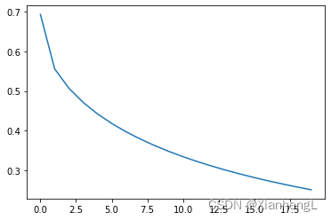
w,b,costs,Y_prediction_test = MyTestModel(train_set_x,train_set_y,test_set_x,test_set_y,2000,0.002)
plot_costs = np.squeeze(costs)
plt.plot(plot_costs)
代价函数曲线:
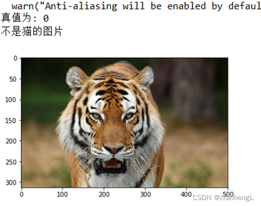
5.图像测试
#测试图片
def isCat(my_image = "my_image.jpg", dirname = "images/"):

    # 初始化图片路径
    fname = dirname + my_image

    # 读取图片
    image = np.array(plt.imread(fname))

    # 将图片转换为训练集一样的尺寸
    num_px = train_set_x_orig.shape[2]
    my_image = skimage.transform.resize(image, output_shape=(num_px,num_px)).reshape((1, num_px*num_px*3)).T

    # 预测
    my_predicted_image = predict(w, b, my_image)

    # 绘图与结果输出
    plt.imshow(image)
    if float(my_predicted_image) == 1.0:
        print('这是一张猫的图片')
    else:
        print('不是猫的图片')

isCat(my_image = "xxx.jpg", dirname="images/")
完整代码:
import numpy as np
import matplotlib.pyplot as plt
import scipy     #数值运算、图像处理
import h5py        #存放数据集和组
import skimage
from scipy import ndimage     #N维图像包
from PIL import Image
from lr_utils import load_dataset
train_set_x_orig, train_set_y, test_set_x_orig, test_set_y, classes = load_dataset()

#降维
train_set_x_flatten = train_set_x_orig.reshape(train_set_x_orig.shape[0],-1).T
test_set_x_flatten = test_set_x_orig.reshape(test_set_x_orig.shape[0],-1).T

#归一化
train_set_x = 1.0*train_set_x_flatten/255
test_set_x = 1.0*test_set_x_flatten/255

'''********搭建神经网络**********'''
def sigmoid(z):
    s = 1 / (1 + np.exp(-z))
    return s

def initialize(n):
    w = np.zeros(shape=(n,1),dtype = np.float32)
    b = 0
    return w,b

def spread(w,b,X,Y):
    #向前传播
    m = X.shape[1]
    A = sigmoid(np.dot(w.T,X)+b)
    J = -1/m * np.sum((Y * np.log(A) + (1-Y) * np.log(1-A)),axis = 1)  #成本函数
    #向后传播
    dw = 1/m * np.dot(X,(A-Y).T)
    db = 1/m * np.sum(A-Y,axis = 1)
    J = np.squeeze(J)    #将cost从矩阵转化为一个实数,从数组中把shape中为1的维度去掉
    return dw,db,J

def gradient_descent(w,b,X,Y,train_times,learning_rate):
    costs = []
    for i in range(train_times):
        dw,db,J = spread(w,b,X,Y)
        w = w -learning_rate * dw
        b = b -learning_rate * db
        #记录成本函数
        if i%100 ==0:
            print('第',i+100,'次的成本函数:',J)
            costs.append(J)
    return w,b,costs

def predict(w,b,X):
    m = X.shape[1]
    Y_prediction = np.zeros((1,m))
    #确保矩阵维数匹配
    w = w.reshape(X.shape[0],1)
    #计算Logistic回归
    A = sigmoid(np.dot(w.T,X) + b)

    for i in range(A.shape[1]):
        if A[0,i] > 0.5:
            Y_prediction[0,i] = 1
        else:
            Y_prediction[0,i] = 0
    #确保矩阵维数正确
    assert(Y_prediction.shape == (1,m))
    return Y_prediction

def MyTestModel(X_train,Y_train,X_test,Y_test,train_times = 100,learning_rate = 0.005):
   #初始化参数
    w,b =initialize(X_train.shape[0])
    #梯度下降训练
    w,b,costs = gradient_descent(w,b,X_train,Y_train,train_times,learning_rate)

    #训练后测试结果
    Y_prediction_train = predict(w,b,X_train)
    Y_prediction_test = predict(w,b,X_test)

    #输出效果
    print('训练集准确率:', '%.2f' % (100 - np.mean(np.abs(Y_prediction_train - Y_train))*100),'%')
    print('测试集准确率:', '%.2f' % (100 - np.mean(np.abs(Y_prediction_test - Y_test))*100),'%')    #np.mean  求取平均值
    print(Y_prediction_test)
    return w,b,costs,Y_prediction_test

#效果测试
w,b,costs,Y_prediction_test = MyTestModel(train_set_x,train_set_y,test_set_x,test_set_y,2000,0.002)
plot_costs = np.squeeze(costs)
plt.plot(plot_costs)

#测试图片
def isCat(my_image = "my_image.jpg", dirname = "images/"):

    # 初始化图片路径
    fname = dirname + my_image

    # 读取图片
    image = np.array(plt.imread(fname))

    # 将图片转换为训练集一样的尺寸
    num_px = train_set_x_orig.shape[2]
    my_image = skimage.transform.resize(image, output_shape=(num_px,num_px)).reshape((1, num_px*num_px*3)).T

    # 预测
    my_predicted_image = predict(w, b, my_image)

    # 绘图与结果输出
    plt.imshow(image)
    if float(my_predicted_image) == 1.0:
        print('这是一张猫的图片')
    else:
        print('不是猫的图片')


 694
694


 被折叠的 条评论
为什么被折叠?
被折叠的 条评论
为什么被折叠?
 到【灌水乐园】发言


