


 文章展示了如何使用Python脚本处理VASP和QE软件产生的能带结构数据,包括读取数据、处理数据、绘制能带图以及标注关键信息。提供的代码包括load_data.py用于数据处理,bandplot_qe.py和bandplot_vasp.py分别用于绘制QE和VASP的能带图。通过这些脚本,用户可以自定义路径并生成能带结构图,对比不同计算结果。
能带数据可以直接用origin画出,同时也可以使用python处理,先对输出文件进行数据处理,读取所需变量,再进行画图,对图像进行标注。
注意事项:
- path地址需要进行相应的修改,并且python文件要放在同一文件目录下。
- VASP的生成文件比较简洁,且自带高对称点坐标和名字。
- QE的输出文件比较乱…而且只能从文件中读取高对称点坐标,坐标名字需要自己输入…
代码结构:
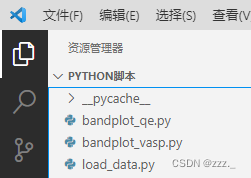
bandplot_qe.py为QE画图,band_vasp.py为VASP画图,load_data.py为处理数据部分。
下面为代码展示,直接复制粘贴就行,注意名字一致。
load_data.py文件
#load_data.py文件
import numpy as np
import re

#加载数据,并将数据按空格和\n分割为单个列表,实现字符串的转换(只含数字)
def process_data_vasp(path):
    file_read=open(path,'r')
    sourceline=file_read.readlines()
    datasets=[]
    for line in sourceline:
        temp1=line.strip()#去掉字符串两端空格和\n
        if(re.search(r'[a-z,A-Z]',temp1)):#去掉含字母的行
            continue
        temp1=temp1.split()#实现空格分割
        temp1 = list(map(float, temp1))
        datasets.append(temp1)
    file_read.close()
    datasets=list(filter(None,datasets))#过滤空值,将返回值转成列表
    datasets=np.asarray(datasets)
    return datasets

#得到k点值和坐标,方便画图标坐标轴
def get_kpoints_vasp(path):
    file_read=open(path,'r')
    sourceline=file_read.readlines()
    datasets=[]
    temp2=[]
    temp3=[]
    for line in sourceline:
        temp1=line.strip()
        if(re.search(r'[0-9]',temp1)):
            temp1=temp1.split()
            temp2.append(temp1[0])
            temp3.append(temp1[1])
    file_read.close()
    temp3=list(map(float,temp3))
    datasets.append(temp2)
    datasets.append(temp3)
    datasets=list(filter(None,datasets))
    return datasets

#用于得到价带最大值和导带最小值
def get_max_negative(datasets):
    temp1=-np.inf
    for i in datasets:
        if i<0:
            if i>temp1:
                temp1=i
    return temp1

def get_min_positive(datasets):
    temp1=np.inf
    for i in datasets:
        if i>0:
            if i<temp1:
                temp1=i
    return temp1

def process_data_qe(path):
    #读取文件,使用with可以自带.close()方法
    with open(path+'bd.dat','r') as file_read1:
        sourceline1=file_read1.readlines()
    with open(path+'bd.dat.gnu','r') as file_read2:
        sourceline2=file_read2.readlines()
    #获取能带数量和数目,数目nks在后边有用
    nbnd_nks=sourceline1[0].strip()#nbnd为能带数量,nks为k点数目
    nbnd_nks=re.sub('[A-Z,a-z,/,&,=]','',nbnd_nks)
    nbnd_nks=nbnd_nks.split()
    nbnd=int(nbnd_nks[0])
    nks=int(nbnd_nks[1])
    #由于bd.dat.gnu每组数据都为正序,所以画图会出现几条从0到最大k点的直线
    #所以将奇数组的序列倒转,即可解决问题(vasp的输出文件BAND.dat即是如此)
    data=[]#输出最终数据
    temp1=[]#用于存放需要倒转的元素
    temp2=[]
    i=-1#记录data的索引,而非sourceline的索引,因为之间差一个空行
    for line in sourceline2:
        line=line.strip()
        if line=='':
            continue
        #data.append(line)
        i=i+1
        if (i//nks)%2==1:
            temp1.append(line)
            continue
        temp1.reverse()
        temp2=temp2+temp1
        temp1=[]
        temp2.append(line)
    #当为奇数组时,会直接跳出循环,忽略最后一组数据,因此下两行代码用于处理最后一组数据
    temp1.reverse()
    temp2=temp2+temp1
    #将字符串转为浮点数
    for i in temp2:
        i=i.split()
        i=list(map(float,i))
        data.append(i)
    #转为numpy的数组,方便索引
    data=np.asarray(data)
    return data

#处理qe文件bands.out,得到k点坐标,同时返回三维坐标和x轴坐标
def get_kpoints_qe(path):
    file_read=open(path+'bands.out')
    sourceline=file_read.readlines()
    data=[]
    for line in sourceline:
        if(re.search('high-symmetry point',line)):
            line=line.strip()#strip之后,line为一个字符串,而不是列表(使用split会生成列表,列表会出错)
            #字符串在某种意义上讲,约等于一维列表,所以输出上一行,会发现是一维列表,但是不会出错
            line=re.sub('[A-Z,a-z,:,-]','',line)#去除字母和':'符号和'-'符号,感觉这个很方便
            line=line.split()#空格分隔
            line=list(map(float,line))#将字符串转为浮点数
            data.append(line)
    data=np.asarray(data)
    return data

#读取费米能级,不得不说,QE确实是一滩狗屎,输出文件乱七八糟,没有vasp简洁
def read_fermi(path):
    with open(path+'vc-relax.out') as file_read:
        sourceline=file_read.readlines()
    feimi=0
    for line in sourceline:
        if(re.search('Fermi energy',line)):
            line=line.strip()
            line=re.sub('[A-Z,a-z]','',line)
            fermi=float(line)
    return fermi

if __name__=="__main__":
    print("this is a python file that processes the data and return something")
bandplot_qe.py
#bandplot_qe.py
#需将下列所需文件放再同一文件目录下
#bands.out读取高对称点
#bd.dat读取能带组数,bd.dat.gnu读取数据
#vc-relax.out用于读取费米能级
import matplotlib.pyplot as plt
import numpy as np
import re
import load_data

path='E:\材料计算\计算结果\SiC\\'
kpoints=load_data.get_kpoints_qe(path)
kpoints_d1=kpoints[:,3]
kpoint_name=[r'${\Gamma}$','M','K',r'${\Gamma}$']#python不能显示罗马字母,因此使用r'${\Gamma}$'来表示
#kpoints_name=[r'${\Gamma}$','M','K']
data=load_data.process_data_qe(path)
data=load_data.process_data_qe(path)

fermi=load_data.read_fermi(path)
x=data[:,0]
y=data[:,1]-fermi
CBM=load_data.get_min_positive(y)
VBM=load_data.get_max_negative(y)
band_gap=CBM-VBM

plt.plot(x,y,'b',lw=0.5)
plt.xlabel("K points")
plt.ylabel("Energy Band(eV)")
plt.xlim(min(kpoints_d1),max(kpoints_d1))#设置坐标轴显示范围,根据KLABELS中的范围设定
plt.xticks(kpoints_d1,kpoints_name)#标k点
plt.axhline(y=0,linestyle='--',color='r',linewidth=0.7)#axh为y轴标虚线
plt.axhline(y=CBM,linestyle='--',color='k',linewidth=0.4)
plt.axhline(y=VBM,linestyle='--',color='k',linewidth=0.4)
plt.axvline(kpoints_d1[1],linestyle='--')#axv为x轴标虚线
plt.axvline(kpoints_d1[2],linestyle='--')

#标注能隙
if band_gap>0:
    plt.title("Band gap="+str(band_gap)[0:8]+" eV")
    plt.fill([kpoints_d1[0],kpoints_d1[-1],kpoints_d1[-1],kpoints_d1[0]],
             [VBM,VBM,CBM,CBM],
             facecolor='pink',
             alpha=0.7)
plt.savefig(path+"bandplot.png",dpi=600)
plt.show()
bandplot_vasp.py
#bandplot_vasp.py
import matplotlib.pyplot as plt
import numpy as np
import re
import load_data

#path='E:\材料计算\计算结果\SbBi\\'
path='E:\材料计算\计算结果\Bi\\'
#path='E:\材料计算\计算结果\BaTiO3\\'
data=load_data.process_data_vasp(path+"BAND.dat")
kpoints=load_data.get_kpoints_vasp(path+"KLABELS")
x=data[:,0]
y=data[:,1]
CBM=load_data.get_min_positive(y)
VBM=load_data.get_max_negative(y)
band_gap=CBM-VBM
plt.plot(x,y,'b',lw=0.5)
plt.xlabel("K points")
plt.ylabel("Energy Band(eV)")
plt.xlim(min(kpoints[1]),max(kpoints[1]))#设置坐标轴显示范围,根据KLABELS中的范围设定
plt.xticks(kpoints[1],kpoints[0])#标k点,[0]为名字,[1]为数字刻度
plt.axhline(y=0,linestyle='--',color='r',linewidth=0.7)#axh为y轴标虚线
plt.axhline(y=CBM,linestyle='--',color='k',linewidth=0.4)
plt.axhline(y=VBM,linestyle='--',color='k',linewidth=0.4)
plt.axvline(kpoints[1][1],linestyle='--')#axv为x轴标虚线
plt.axvline(kpoints[1][2],linestyle='--')
if band_gap>0:
    plt.title("Band gap="+str(band_gap)[0:8]+" eV")
    plt.fill([kpoints[1][0],kpoints[1][-1],kpoints[1][-1],kpoints[1][0]],
             [VBM,VBM,CBM,CBM],
             facecolor='pink',
             alpha=0.7)
plt.savefig(path+"bandplot.png",dpi=600)
plt.show()
结果展示
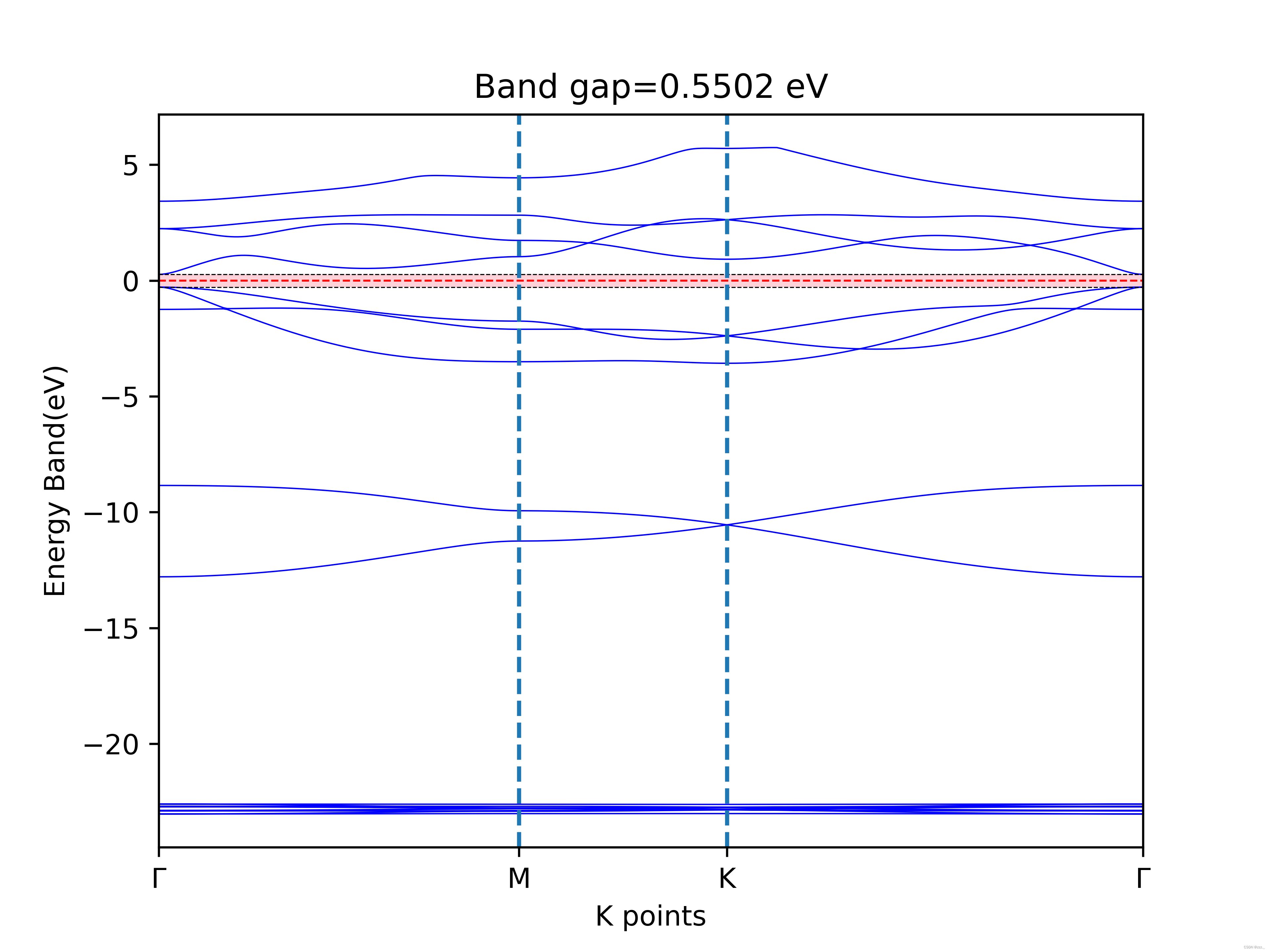
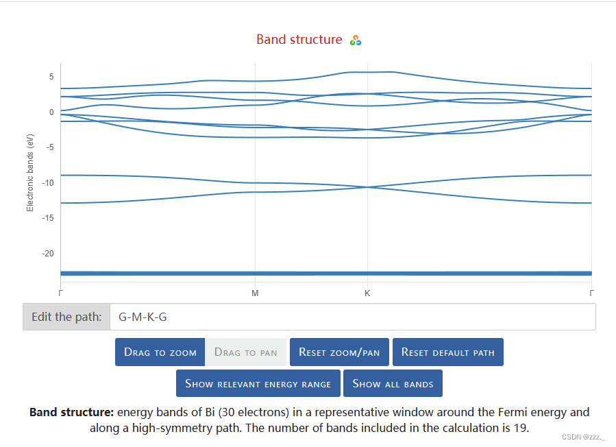
以Bi的平面结构为例:第一张为自己计算结果,第二张为网络上计算结果,可以看出结果高度一致
最新进展
直接把代码克隆到gitee里了(好方便),移步数据画图代码,增加了面向对象的结构,可以在同一张画布上画多个数据结果图像(因为只使用plt.plot()的话实在过于麻烦),增加了剪切费米能级附近的功能,并且有些能带数据会部分大于费米能级,部分小于费米能级,增加判别价带导带的功能。
下面是效果图像:


 836
836

 被折叠的 条评论
为什么被折叠?
被折叠的 条评论
为什么被折叠?
 到【灌水乐园】发言


