VASP+AMSET plot 绘制能带图

W Li DFT计算杂谈 2023-07-28 00:32

收录于合集

#amset

#vasp20个

#能带

#绘图

前期已经介绍过有关AMSET与vasp对接计算材料能带、态密度、弹性常数、电运输性质（包括电导率，Seebeck系数，迁移率等）内容。

笔者在计算过程中发现amset所具有的plot功能比较丰富，且具有简易操作和节省计算资源的优点，所以在这里向大家介绍。

首先运行amset plot命令

mset plot
Usage: amset plot [OPTIONS] COMMAND [ARGS]...
  Plot AMSET results, including scattering rates and band structures
Options:  -h, --help  Show this message and exit.
Commands:  band         Plot interpolate band structure from vasprun file  convergence  Plot transport properties  lineshape    Plot band structures with electron lineshape  mobility     Plot mobility in more detail  rates        Plot scattering rates  transport    Plot transport properties

可看到其可根据已有计算基础和输入文件，自定义绘制包括能带结构（根据已有计算vasprun.xml，可包括能态密度）、电运输性质（包括Seebeck系数、电导率、迁移率，在指定掺杂浓度即固定的载流子浓度的基础上不同温度下的曲线图）、 更为详细的载流子迁移率和不同的散射机制。 

命令使用格式为：amset plot [OPTIONS] COMMAND [ARGS]

这里查看amset plot band的使用帮助

amset plot band -h
Usage: amset plot band [OPTIONS] FILENAME
  Plot interpolate band structure from vasprun file
Options:  -l, --line-density FLOAT        band structure line density  --emin FLOAT                    minimum energy limit  --emax FLOAT                    maximum energy limit  --symprec FLOAT                 interpolation factor  --print-log / --no-print-log    whether to print interpolation log  --kpath [pymatgen|seekpath]     k-point path type  --kpoints K                     manual k-points list [e.g. '0 0 0, 0.5 0 0']  --labels L                      labels for manual kpoints [e.g. '\Gamma,X']  --interpolation-factor FLOAT    BoltzTraP interpolation factor  --energy-cutoff FLOAT           interpolation energy cutoff in eV  -z, --zero-weighted-kpoints [keep|drop|prefer]                                  how to process zero-weighted k-points  --plot-dos                      whether to also plot the density of states  --dos-kpoints TEXT              k-point length cutoff or mesh for density of                                  states
  --dos-estep FLOAT               dos energy step size  --dos-aspect FLOAT              aspect ratio for the density of states  --no-zero-to-efermi             don't set the Fermi level to zero  --vbm-cbm-marker                add a marker at the CBM and VBM  --stats                         print effective mass and band gap  --width FLOAT                   figure width [default: 6]  --height FLOAT                  figure height [default: 6]  -p, --prefix TEXT               output filename prefix  --directory PATH                file output directory  --format [pdf|png|svg|jpg]      image format  --style TEXT                    path to matplotlib style specification  --no-base-style                 don't apply base style  -h, --help                      Show this message and exit.

可见可根据需求自行设置，绘制自定义能带结构图片。

其中比较突出的功能点为：

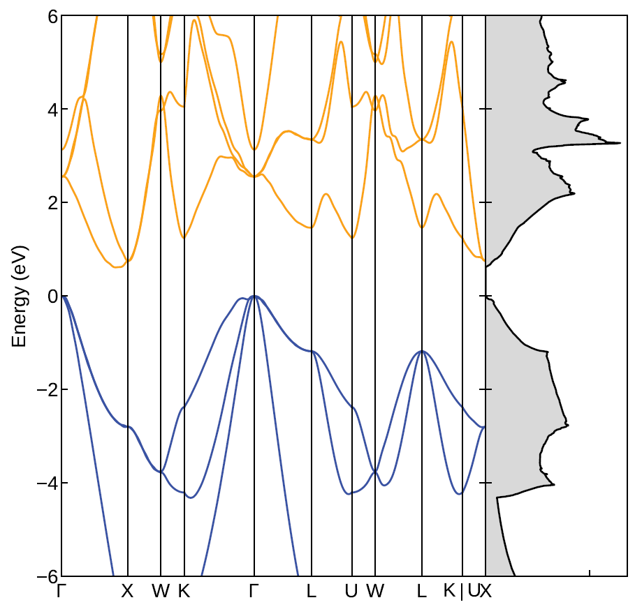
--plot-dos  可在绘制能带的同时绘制相应的能态密度；

--no-zero-to-efermi ，不再以费米能级为0点，可直接获得能带尤其是导带底价带顶的能量位置（对于形变势计算比较有用）；

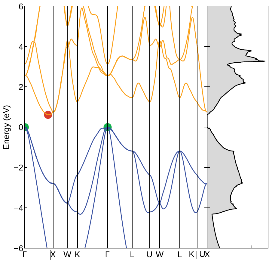
--vbm-cbm-marker ，可直接显示导带底和价带顶位置；

 --stats    ，在绘制能带图后计算电子有效质量和计算带隙；

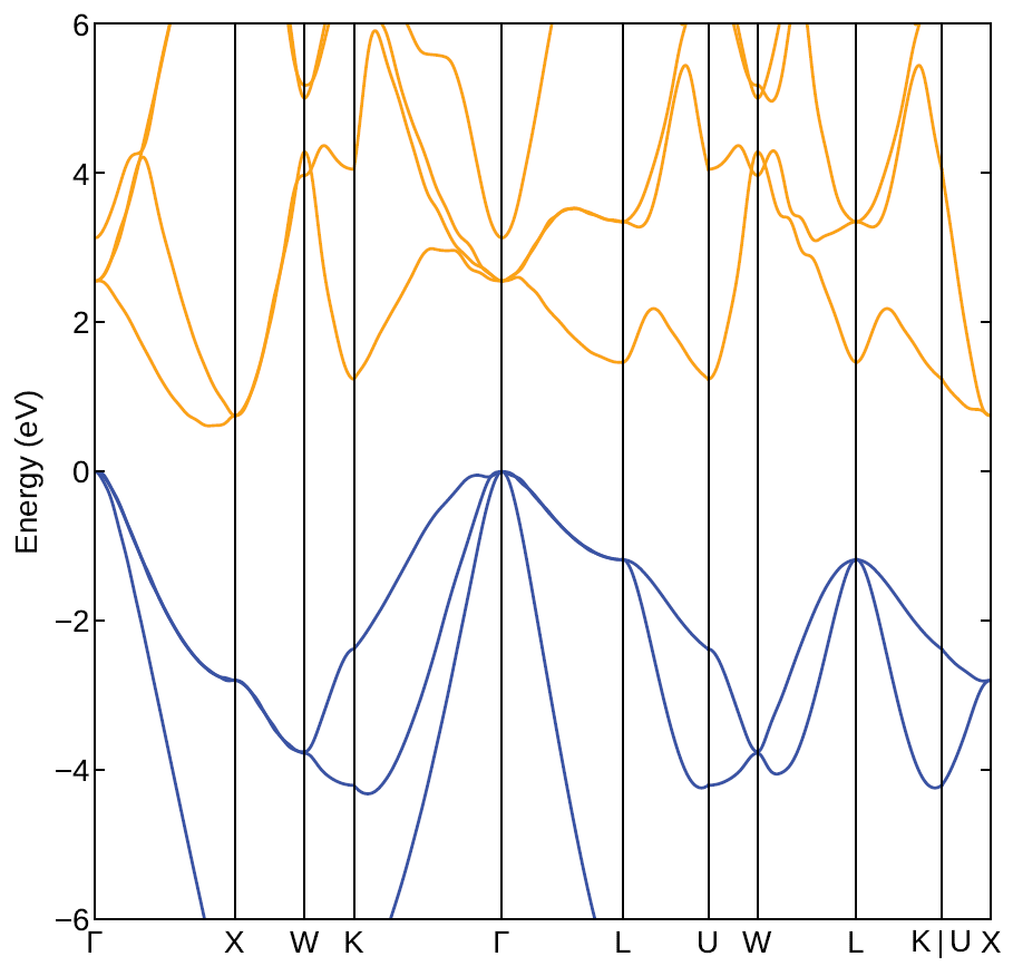
amset plot band  vasprun.xml

绘制得到的example里Si的能带结构

添加了 --stats  参数得到的带隙和有效质量数据

Band structure information~~~~~~~~~~~~~~~~~~~~~~~~~~
Indirect band gap: 0.615 eVDirect band gap: 2.556 eV  k-point: [0.00, 0.00, 0.00]  k-point indices: 0, 339, 340  Band indices: 2, 6
Valence band maximum:  Energy: 5.618 eV  k-point: [0.00, 0.00, 0.00]  k-point location: \Gamma  k-point indices: 0, 339, 340  Band indices: 1, 2, 3
Conduction band minimum:  Energy: 6.232 eV  k-point: [0.41, 0.00, 0.41]  k-point location: between \Gamma-X  k-point indices: 94  Band indices: 4
Using nonparabolic fitting of the band edges
Hole effective masses:  m_h: -0.104 | band 1 | [0.00, 0.00, 0.00] (\Gamma) -> [0.50, 0.00, 0.50] (X)  m_h: -0.100 | band 1 | [0.00, 0.00, 0.00] (\Gamma) -> [0.38, 0.38, 0.75] (K)  m_h: -0.098 | band 1 | [0.00, 0.00, 0.00] (\Gamma) -> [0.50, 0.50, 0.50] (L)  m_h: -1.118 | band 2 | [0.00, 0.00, 0.00] (\Gamma) -> [0.50, 0.00, 0.50] (X)  m_h: -1.490 | band 2 | [0.00, 0.00, 0.00] (\Gamma) -> [0.38, 0.38, 0.75] (K)  m_h: -1.694 | band 2 | [0.00, 0.00, 0.00] (\Gamma) -> [0.50, 0.50, 0.50] (L)  m_h: -0.285 | band 3 | [0.00, 0.00, 0.00] (\Gamma) -> [0.50, 0.00, 0.50] (X)  m_h: -0.304 | band 3 | [0.00, 0.00, 0.00] (\Gamma) -> [0.38, 0.38, 0.75] (K)  m_h: -0.309 | band 3 | [0.00, 0.00, 0.00] (\Gamma) -> [0.50, 0.50, 0.50] (L)
Electron effective masses:  m_e: 0.976 | band 4 | [0.41, 0.00, 0.41] -> [0.50, 0.00, 0.50] (X)  m_e: 0.744 | band 4 | [0.41, 0.00, 0.41] -> [0.00, 0.00, 0.00] (\Gamma)

添加了--plot-dos 绘制的能带和能态密度的图片

 添加 --vbm-cbm-marker，突出显示导带底和价带顶。

绘制得到的具有electron lineshape的能带结构，需要前置执行amset run计算，详细请参考公众号有关amset计算的文章。

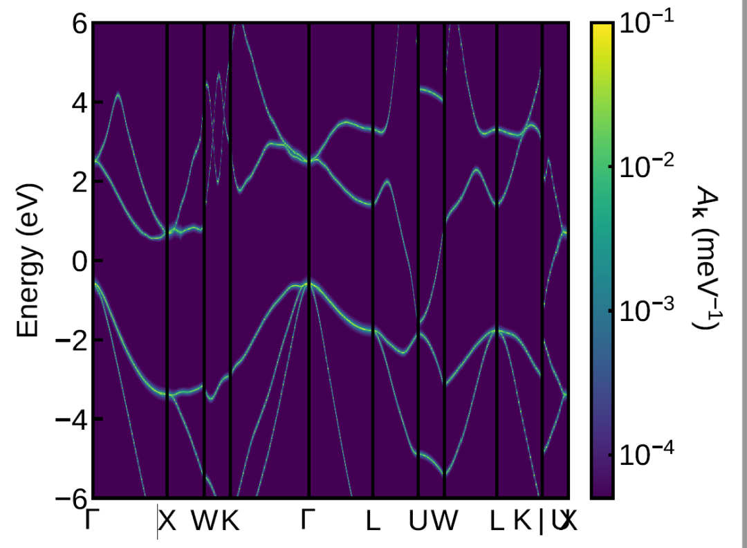
执行命令为

amset plot lineshape mesh_105x105x105.h5 --emin=-6 --emax=6

mesh文件名请根据实际情况修改。

本号不定期发布有关DFT计算相关内容，主题多变且不固定。

欢迎分享推送，将教程与经验传播给需要的人。

如对教程内容有疑问，或者有需要咨询，可后台留言或联系作者：hn_87165

同时如想加入交流群，也可添加作者并说明。

最后，如果您有DFT计算相关经验，愿意写相关的教程，也可以联系作者投稿。

愿有所成

引喻失义   妄自菲薄