【pytorch01】简单回归问题

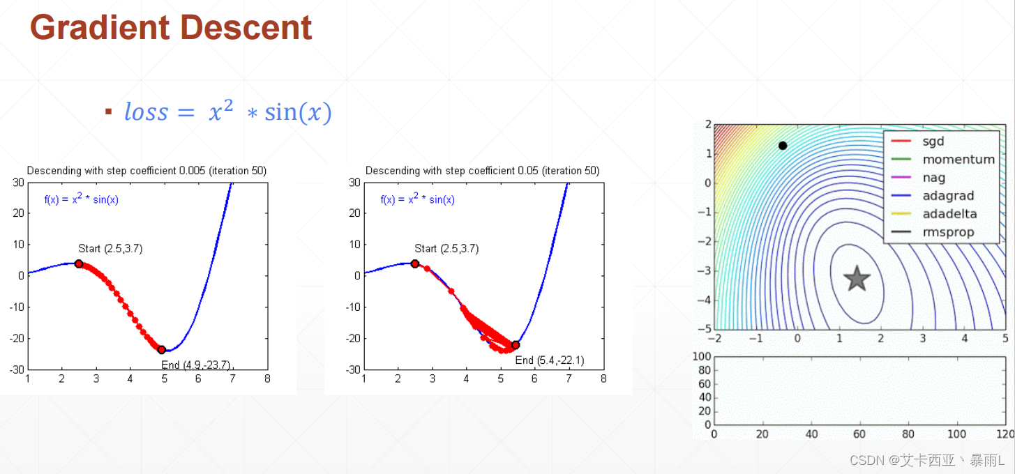
1.梯度下降（Gradient Descent）

$y=x^2\ast sin(x)$
$y^{\prime }=2\ast x\ast sin(x)+x^2\ast cos(x)$
求最小值要求导

梯度下降定义：梯度下降要迭代计算，每一次得到一个导数以后，用原来的x减去该x处导数的值，得到一个新的x的值就是这样一个迭代的过程

$x_t=x_{t-1}-\eta \frac{\partial y}{\partial x_{t-1}}$

η就是learning rate（学习率），可以通过调整学习率够使目标函数在合适的时间内收敛到局部最小值。

• $y=w\ast x+b$
  • $1.567=w\ast 1+b$
  • $3.043=w\ast 2+b$

w = 1.477
b = 0.089
通过消元法，此时w和b是一个准确解，被称之为Closed Form Solution

其实现实生活中可以精确求解的东西不多，我们现实生活中拿到的数据都是有一定偏差的，因此对于实际的问题，与其说求一个Closed Form Solution（封闭解），不如求得一个近似解，这个近似解在经验上可行，这样就可以达到我们的目的

用高斯噪声（均值为0.01，方差为1）模仿偏差（现实生活中拿到的数据都是带有一定噪声的）
$y=w\ast x+b+ϵ$
$ϵ\sim N(0.01,1)$
$$\begin{gathered} 1.567=w^{\star }1+b+eps \\ 3.043=w^{\star }2+b+eps \\ 4.519=w^{\star }3+b+eps \\ ... \end{gathered}$$
观测一组数据，通过观测这一组数据来求解，这一组数据中整体表现比较好的解，虽然不是Closed Form Solution，但是证明了有良好的表现，可以达到需求。

$y=x^2\ast sin(x)$使用梯度下降算法是求这个函数的最小值

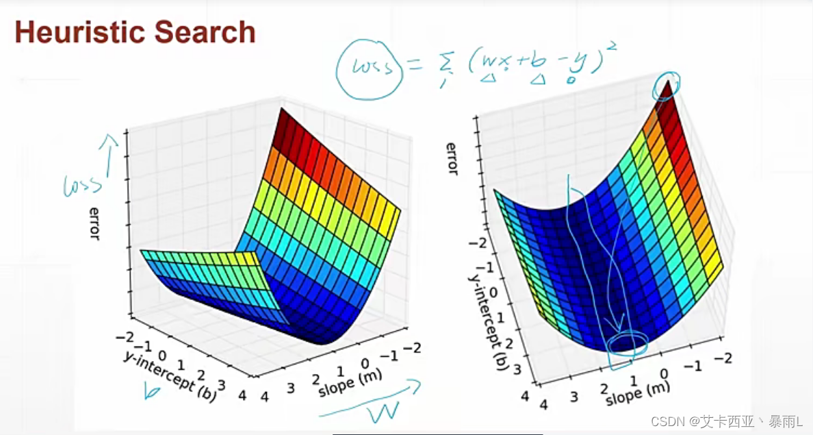
但是对于$y=w\ast x+b$这个方程来说并不是要求y的最小值，而是要求真实的y和$w\ast x+b$的差最小，因为希望$w\ast x+b$更加接近真实的y的值

可以通过求$loss=(w\ast x+b-y{)}^2$的极小值，可以达到接近的目的，获取此时的w和b的值

2.实战

$loss=(WX+b-y{)}^2$

# 返回average loss
def compute_error_for_line_given_points(w,b,points):
    lossTotal = 0
    for i in range(len(points)):
        x = points[i,0]
        y = points[i,1]
        lossTotal += (y - (w * x + b))** 2
    return lossTotal / float(len(points))

$w^{\prime }=w-lr\ast \frac{\nabla loss}{\nabla w}$

# 要求loss的极小值，对w和b分别梯度下降
def step_gradient(b_current,w_current,points,learningRate):
    b_gradient = 0
    w_gradient = 0
    N = float(len(points))
    for i in range(len(points)):
        x = points[i, 0]
        y = points[i, 1]
        # loss函数分别对w和b求导
        # 多了N的原因是因为对所有点的导数累加起来，这样就不用做average了
        # 此时获得的w和b是所有点average之后的梯度
        w_gradient += -(2/N) * x * (y - (w_current * x + b_current))
        b_gradient += -(2/N) * (y - (w_current * x + b_current))
    new_b = b_current - (learningRate * b_gradient)
    new_w = w_current - (learningRate * w_gradient)
    return [new_w,new_b]

经过多次梯度下降得到最优解

def gradient_descent_runner(points,starting_w,starting_b,
                            learning_rate,num_iterations):
    w = starting_w
    b = starting_b
    for i in range(num_iterations):
        w,b = step_gradient(w,b,np.array(points),learning_rate)
    return [w,b]

def run():
    points = np.genfromtxt("data.csv",delimiter=",")
    print(points[:10])
    learning_rate = 0.0001
    initial_w = 0
    initial_b = 0
    num_iterations = 1000
    print("Starting gradient descent at w = {0},b = {1},error = {2}"
          .format(initial_w,initial_b,compute_error_for_line_given_points(initial_w,initial_b,points)))

    print("Running...")
    [w,b] = gradient_descent_runner(points,initial_w,initial_b,learning_rate,num_iterations)
    print("After {0} iterations w = {1},b = {2},error = {3}"
          .format(num_iterations,w, b,
                  compute_error_for_line_given_points(w, b, points)))

if __name__ == '__main__':
    run()

最终的数据与Closed Form Solution非常接近