Seurat 源码学习之VlnPlot

今天很好奇Seurat里的Vlnplot是怎么画的，花了一个上午研究一下这个画图，其实还是很简单的哈, 以官网的pbmc3k为例

#
library(dplyr)
library(Seurat)
library(patchwork)
setwd("/Users/xiaokangyu/Desktop/Seurat_raw_code/")
pbmc.data = Read10X("/Users/xiaokangyu/Desktop/test_dataset/pbmc_3k/filtered_gene_bc_matrices/hg19/")

pbmc = CreateSeuratObject(counts = pbmc.data,project = "pbmc3k",min.cells=3,min.features = 200)
pbmc

pbmc[["percent.mt"]] <- PercentageFeatureSet(pbmc, pattern = "^MT-")

pbmc <- subset(pbmc, subset = nFeature_RNA > 200 & nFeature_RNA < 2500 & percent.mt < 5)

pbmc <- NormalizeData(pbmc)

pbmc <- FindVariableFeatures(pbmc, selection.method = "vst", nfeatures = 2000)

all.genes <- rownames(pbmc)

pbmc <- ScaleData(pbmc, features = all.genes)

pbmc <- RunPCA(pbmc, features = VariableFeatures(object = pbmc))

pbmc <- FindNeighbors(pbmc, dims = 1:10)

pbmc <- FindClusters(pbmc, resolution = 0.5)

pbmc <- RunUMAP(pbmc, dims = 1:10)

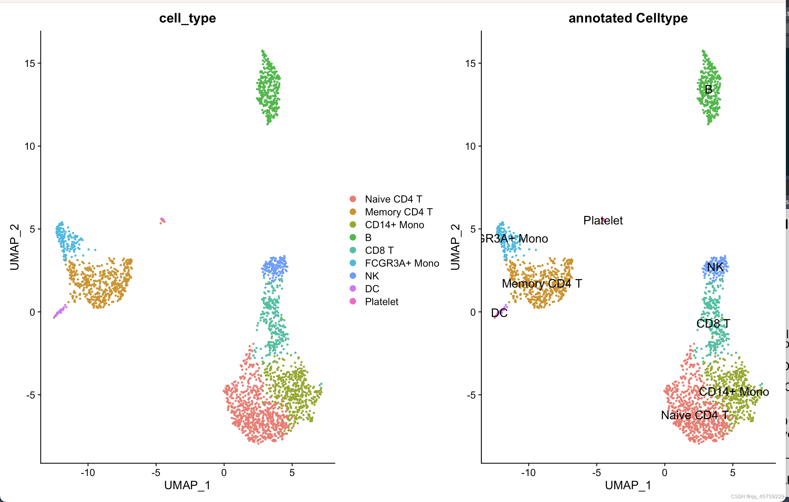
new.cluster.ids <- c("Naive CD4 T", "Memory CD4 T", "CD14+ Mono", "B", "CD8 T", "FCGR3A+ Mono", "NK", "DC", "Platelet")

names(new.cluster.ids) <- levels(pbmc)

pbmc <- RenameIdents(pbmc, new.cluster.ids)

pbmc[['cell_type']] <- pbmc@active.ident

levels(pbmc)

saveRDS(pbmc, file = "./pbmc.rds")

# p =DimPlot(pbmc, reduction = "umap", group.by = "cell_type")#画batch图
# print(p)
# 
# pp=DimPlot(pbmc, reduction = "umap", group.by = "cell_type", label.size = 5,label=T)+ggtitle("annotated Celltype")+NoLegend()
# print(pp)
# 
# print(p+pp)
# p1=FeaturePlot(pbmc, features = c("MS4A1", "GNLY", "CD3E", "CD14", "FCER1A", "FCGR3A", "LYZ", "PPBP",
#                                   "CD8A"))
# 
# p2=FeaturePlot(pbmc, features = c("MS4A1", "CD79A"))
# print(p2)
# 
# p3=VlnPlot(pbmc, features = c("MS4A1", "CD79A"))

p4 = VlnPlot(pbmc,features = c("MS4A1"))

print(p4)
# pbmc@active.assay

结果如下

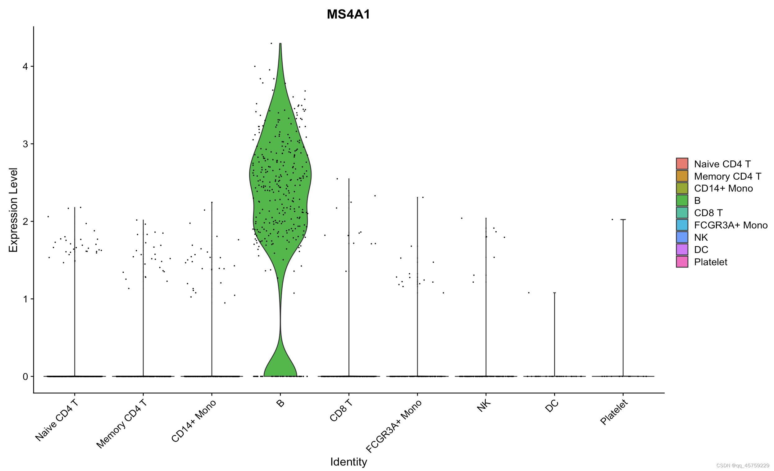
可以看到这个结果很好哈，现在研究这个小提琴图是怎么画的

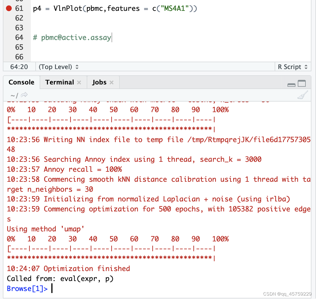
首先注意一点本地mac电脑可以直接调试，而服务器的rstudio打上断点后没有调试的相关按钮，很奇怪
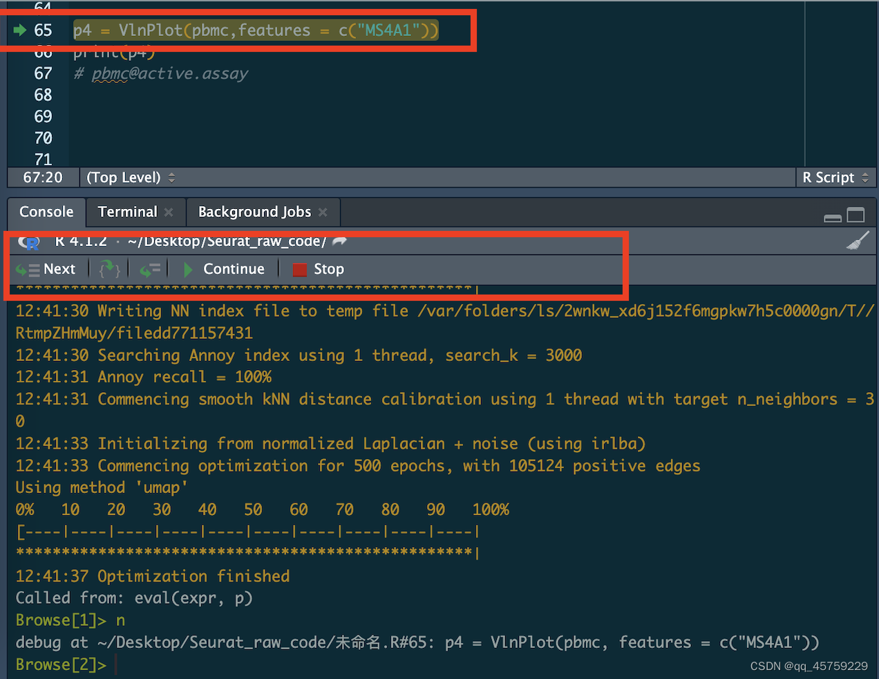而在服务器上

注意在R里的调试有一个好处，虽然我直接安装了Seurat,直接使用调试按钮直接进入函数，但是python里有的包你是进不去的，首先进入的
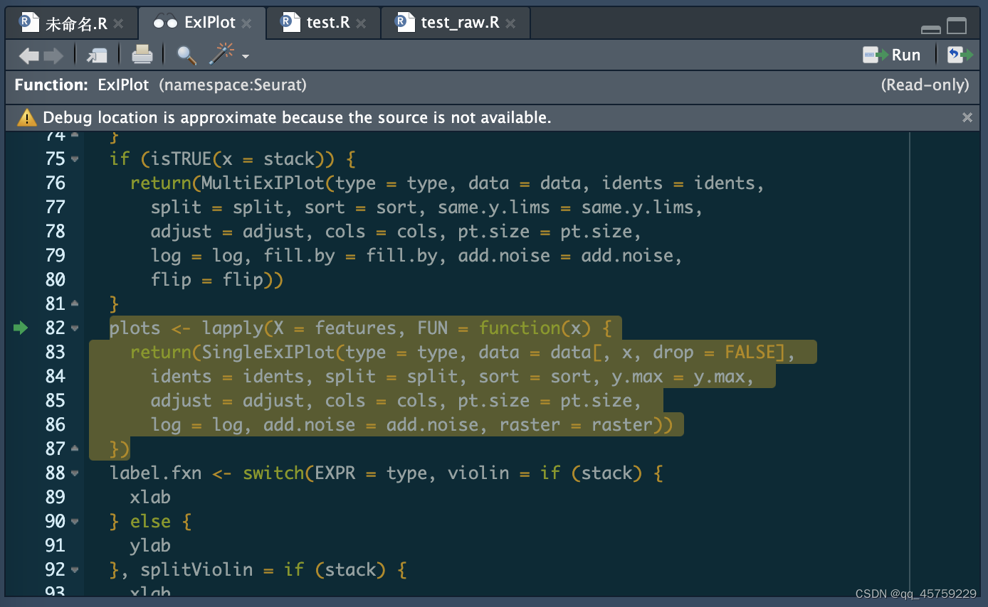
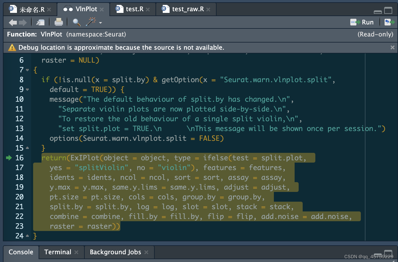可以看到Vlnplot调用的是ExIplot函数，接着调用的是SingleExIPlot函数
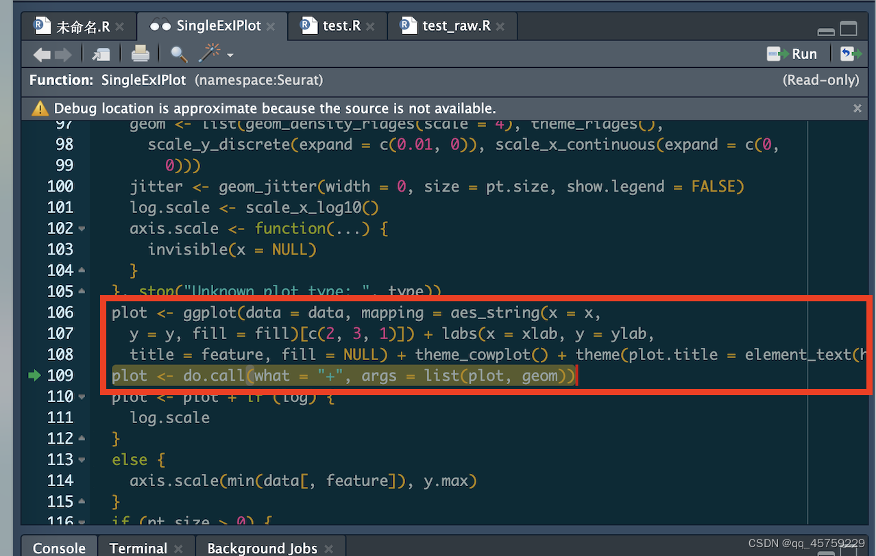这里可以看到真正的画图函数，代码还是很简单的

下面是我自己复现的代码

rm(list=ls())
library(Seurat)
library(ggplot2)
library(cowplot)

pbmc = readRDS("./pbmc.rds")
set.seed(42)
feature ="MS4A1"
data_all = pbmc@assays$RNA@data # 取出来上dgcMatrix是稀疏矩阵，没法取行列
data_df = data.frame(data_all)
data = data.frame(t(data_df[feature,])) # 取feature 基因对应的表达
data$ident =pbmc@meta.data$cell_type # 我这里发现一个R的bug,就是对于因子类型的变量
#如果写入csv文件再读取,那么这个factor对应的level的顺序可能会自己变化，不再是开始保存时的结果了，
#如果要保存level对应的信息时，还是应该使用saveRDS而不是write.csv

noise <- rnorm(n = length(x = data[, feature]))/1e+05
data[, feature] <- data[, feature] + noise

pt.size = 0.1154295
x="ident"
y="`MS4A1`"
fill ="ident"
xlab="Identity"
feature = "MS4A1"
ylab ="Expression Level"

jitter <- geom_jitter(height = 0, size = pt.size, 
                      show.legend = FALSE)
plot <- ggplot(data = data, mapping = aes_string(x = x, 
                                                 y = y, fill = fill)[c(2, 3, 1)]) + labs(x = xlab, y = ylab, 
                                                                                         title = feature, fill = NULL) + theme_cowplot() + theme(plot.title = element_text(hjust = 0.5))

geom <- list(geom_violin(scale = "width", adjust = 1, 
                         trim = TRUE), theme(axis.text.x = element_text(angle = 45, 
                                                                        hjust = 1)))

plot <- do.call(what = "+", args = list(plot, geom))

plot = plot + jitter
print(plot)

这个结果和Seurat画出来的是一样的，嘿嘿

我的环境如下

sessionInfo()
R version 4.1.2 (2021-11-01)
Platform: x86_64-apple-darwin17.0 (64-bit)
Running under: macOS 13.1

Matrix products: default
LAPACK: /Library/Frameworks/R.framework/Versions/4.1/Resources/lib/libRlapack.dylib

locale:
[1] en_US.UTF-8/en_US.UTF-8/en_US.UTF-8/C/en_US.UTF-8/en_US.UTF-8

attached base packages:
[1] stats4    stats     graphics  grDevices utils     datasets  methods   base     

other attached packages:
 [1] cowplot_1.1.1               patchwork_1.1.2             SeuratObject_4.1.3         
 [4] Seurat_4.3.0                dplyr_1.1.0                 ggplot2_3.4.1              
 [7] splatter_1.18.2             SingleCellExperiment_1.16.0 SummarizedExperiment_1.24.0
[10] Biobase_2.54.0              GenomicRanges_1.46.1        GenomeInfoDb_1.30.1        
[13] IRanges_2.28.0              S4Vectors_0.32.4            BiocGenerics_0.40.0        
[16] MatrixGenerics_1.6.0        matrixStats_0.63.0         

loaded via a namespace (and not attached):
  [1] ggbeeswarm_0.7.1       Rtsne_0.16             colorspace_2.0-3      
  [4] deldir_1.0-6           ellipsis_0.3.2         ggridges_0.5.4        
  [7] XVector_0.34.0         rstudioapi_0.14        spatstat.data_3.0-0   
 [10] farver_2.1.1           leiden_0.4.3           listenv_0.9.0         
 [13] ggrepel_0.9.2          fansi_1.0.3            R.methodsS3_1.8.2     
 [16] codetools_0.2-18       splines_4.1.2          polyclip_1.10-4       
 [19] jsonlite_1.8.4         ica_1.0-3              cluster_2.1.2         
 [22] R.oo_1.25.0            png_0.1-8              uwot_0.1.14           
 [25] shiny_1.7.4            sctransform_0.3.5      spatstat.sparse_3.0-0 
 [28] compiler_4.1.2         httr_1.4.4             backports_1.4.1       
 [31] Matrix_1.5-1           fastmap_1.1.0          lazyeval_0.2.2        
 [34] cli_3.6.0              later_1.3.0            htmltools_0.5.4       
 [37] tools_4.1.2            igraph_1.3.5           gtable_0.3.1          
 [40] glue_1.6.2             GenomeInfoDbData_1.2.7 RANN_2.6.1            
 [43] reshape2_1.4.4         Rcpp_1.0.10            scattermore_0.8       
 [46] vctrs_0.5.2            spatstat.explore_3.0-5 nlme_3.1-153          
 [49] progressr_0.13.0       lmtest_0.9-40          spatstat.random_3.0-1 
 [52] stringr_1.5.0          globals_0.16.2         mime_0.12             
 [55] miniUI_0.1.1.1         lifecycle_1.0.3        irlba_2.3.5.1         
 [58] goftest_1.2-3          future_1.30.0          zlibbioc_1.40.0       
 [61] MASS_7.3-54            zoo_1.8-11             scales_1.2.1          
 [64] promises_1.2.0.1       spatstat.utils_3.0-1   parallel_4.1.2        
 [67] RColorBrewer_1.1-3     reticulate_1.27        pbapply_1.6-0         
 [70] gridExtra_2.3          ggrastr_1.0.1          stringi_1.7.8         
 [73] checkmate_2.1.0        BiocParallel_1.28.3    rlang_1.1.0           
 [76] pkgconfig_2.0.3        bitops_1.0-7           lattice_0.20-45       
 [79] ROCR_1.0-11            purrr_1.0.1            tensor_1.5            
 [82] labeling_0.4.2         htmlwidgets_1.6.1      tidyselect_1.2.0      
 [85] parallelly_1.33.0      RcppAnnoy_0.0.20       plyr_1.8.8            
 [88] magrittr_2.0.3         R6_2.5.1               generics_0.1.3        
 [91] DelayedArray_0.20.0    DBI_1.1.3              withr_2.5.0           
 [94] pillar_1.8.1           fitdistrplus_1.1-8     survival_3.2-13       
 [97] abind_1.4-5            RCurl_1.98-1.9         sp_1.5-1              
[100] tibble_3.2.1           future.apply_1.10.0    crayon_1.5.2          
[103] KernSmooth_2.23-20     utf8_1.2.2             spatstat.geom_3.0-3   
[106] plotly_4.10.1          locfit_1.5-9.7         grid_4.1.2            
[109] data.table_1.14.6      digest_0.6.31          xtable_1.8-4          
[112] tidyr_1.3.0            httpuv_1.6.7           R.utils_2.12.2        
[115] munsell_0.5.0          beeswarm_0.4.0         viridisLite_0.4.1     
[118] vipor_0.4.5