GCN详解

小菜0-o

已于 2023-10-07 22:10:47 修改

阅读量249

点赞数

分类专栏：图神经网络文章标签： python

于 2023-10-06 14:39:45 首次发布

本文链接：https://blog.csdn.net/qq_45895217/article/details/133281392

版权

图神经网络专栏收录该内容

6 篇文章 4 订阅

订阅专栏

$\vec{a}$ 向量
$\overline{a}$ 平均值
$\underline{a}$ 下横线
$\widehat{a}$ (线性回归，直线方程) y尖
$\widetilde{a}$
$\dot{a}$ 一阶导数
$\ddot{a}$ 二阶导数

GCN原理本质大白话解释

GCN和CNN的想法差不多，CNN是通过一个卷积核聚合某个像素点其他周围点的信息，来聚合邻居，GCN是通过邻接矩阵（带自环的）来聚合邻居节点的信息。

在这里插入图片描述
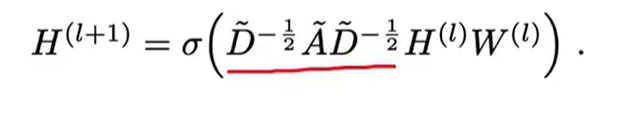
H^(l)表示l层的节点的特征
W^(l)表示l层的参数
$\widetilde{D}$ 表示度矩阵，体现每个节点都度。是个主对角矩阵。
$\widetilde{A}$ 是图的邻接矩阵加上单位矩阵，I是E是单位阵

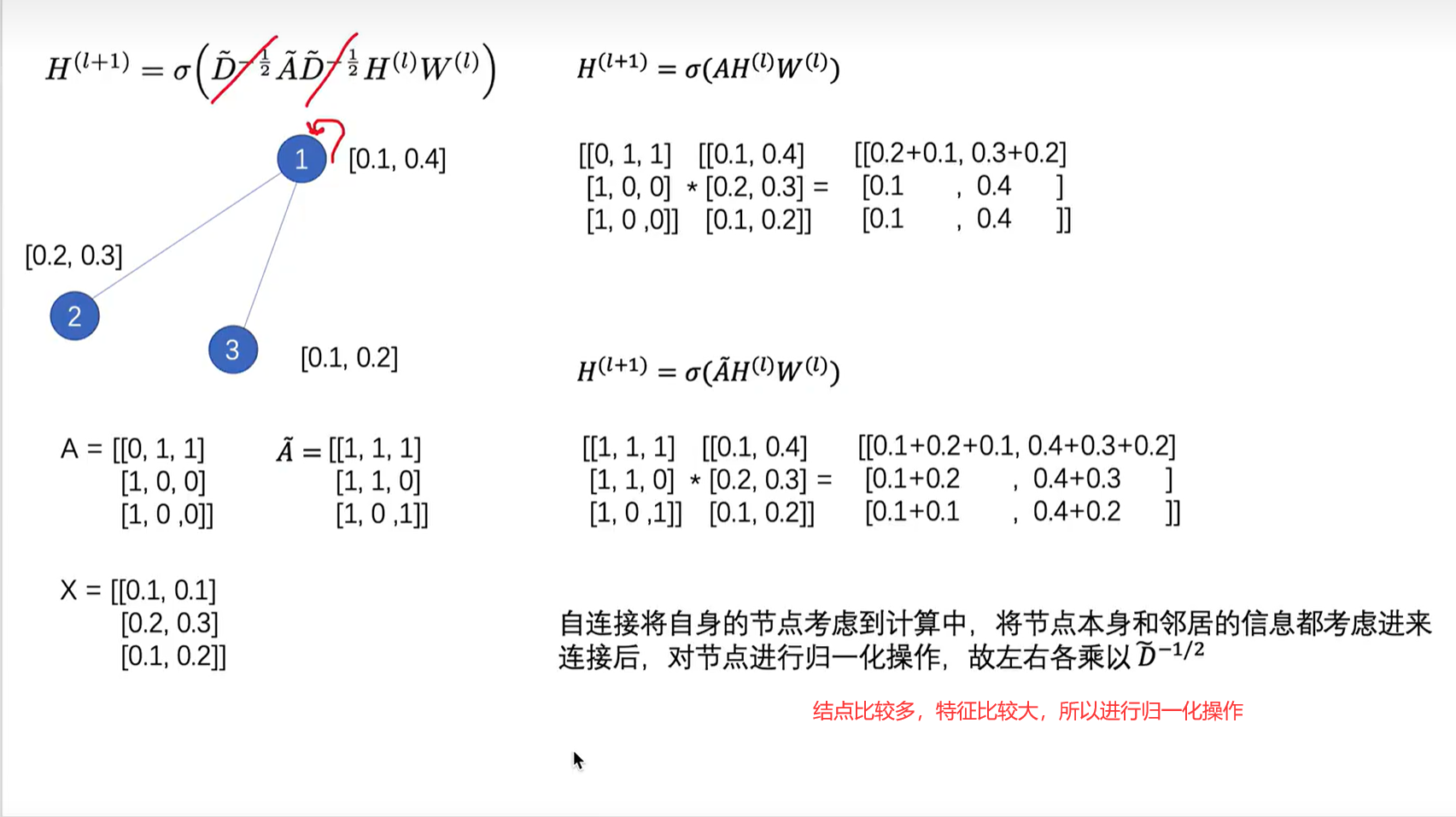
上图中，X是三个节点的特征向量，1节点的特征向量是[0.1, 0.1]

在这里插入图片描述
上图中，Z=f(X, A) 表示具有两层GCN层网络。第一层的参数是W⁽⁰⁾，激活函数是ReLU, 第二层的参数是W¹，激活函数是softmax
如果最后一层的gcn的隐藏层特征数不等于类别数，则在其后面添加一个全连接层。此时的gcn层相当于一个特征提取器，再经过全连接层当作分类器，最后得到的输出层个数等于类别数。

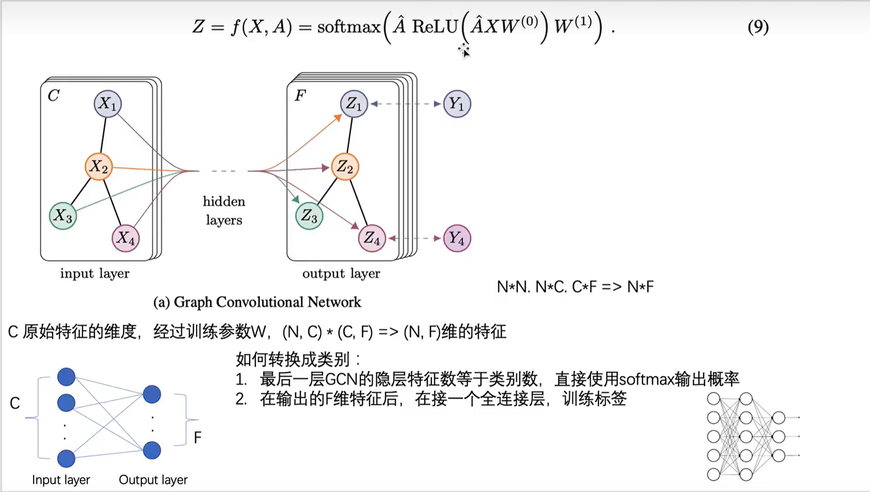
$\widehat{A}$ 为归一化后的 $\widehat{A}$ = $\widetilde{D}$ ^-0.5* $\widehat{A}$ * $\widetilde{D}$ ^-0.5。这里的 $\widehat{A}$ 就是 $\widetilde{L}~sym~$ ，即归一化后的拉普拉斯矩阵
X 是输入值，W⁽⁰⁾是0层的参数值。

在这里插入图片描述
参考文章 & 视频
最通俗易懂的图神经网络（GCN）原理详解

GCN视频讲解

GCN完整代码


# 代码清单1-CoraData类的定义
import itertools
import os
import os.path as osp
import pickle
import urllib
from collections import namedtuple
import numpy as np
import scipy.sparse as sp
import torch
import torch.nn as nn
import torch.nn.functional as F
import torch.nn.init as init
import torch.optim as optim
from matplotlib import pyplot as plt
from sklearn.manifold import TSNE

# 用于保存处理好的数据
Data = namedtuple('Data', ['x', 'y', 'adjacency', 'train_mask', 'val_mask', 'test_mask'])   # 元组，每一个元组都有属性
class CoraData(object):
    download_url = 'https://github.com/kimiyoung/planetoid/tree/master/data/'
    filenames = ["ind.cora.{}".format(name) for name in
                    ['x', 'tx', 'allx', 'y', 'ty', 'ally', 'graph', 'test.index']]
    def __init__(self, data_root='cora', rebulid=False):
        """
        包括数据下载、处理、加载等功能
        当数据的缓存文件存在时，将使用缓存文件，否则将下载、处理并缓存到磁盘
        :param data_root:  存放数据的目录，原始数据的路径：{data_root}/raw
        缓存数据路径：{data_root}/processed_cora.pkl
        :param rebulid: 是否需要重新构建数据集。为True时，如果缓存数据存在也会重建数据
        """
        self.data_root = data_root      # 根路径
        save_file = osp.join(self.data_root, "processed_cora.kpl")
        if osp.exists(save_file) and not rebulid:       # 需要重新下载
            print("Using Cached file:{}".format(save_file))
            self._data = pickle.load(open(save_file, 'rb'))
        else:       # 需要重新下载
            self.maybe_download()
            self._data = self.process_data()
            with open(save_file, 'wb') as f:
                pickle.dump(self.data, f)
            print("Cached file:{}".format(save_file))
    @property       # 加了这个后，方法可以像属性一样调用，不用加括号
    def data(self):
        """
        :return: 返回Data数据对象，包括x, y, adjacency, train_mask, val_mask, test_mask
        """
        return self._data   # self.process_data()
    def maybe_download(self):
        save_path = os.path.join(self.data_root, "raw")
        for name in self.filenames:
            if not osp.exists(osp.join(save_path, name)):
                self.download_data(
                    "{}/ind.cora.{}".format(self.download_url, name), save_path)
    @staticmethod
    def download_data(url, save_path):
        """数据下载工具，当原始数据不存在时将会进行下载"""

        if not os.path.exists(save_path):
            os.makedirs(save_path)
        data = urllib.request.urlopen(url)
        filename = os.path.splitext(url)    # 获取文件名

        with open(osp.join(save_path, filename), 'wb') as f:
            f.write(data.read())        # 从data中读取内容，并写入
        return True

    # 代码清单2-Cora数据处理
    def process_data(self):
        """
        处理数据，得到节点特征和标签，邻接矩阵，训练集，验证集和测试集
        :return:
        """
        print("Process data....")
        """
        x:训练集节点特征向量
        tx : 测试集节点特征向量
        allx :可以理解为除测试集以外的其他节点特征集合
        y : one-hot表示的训练节点的标签
        ty : one-hot表示的测试节点的标签
        ally : one-hot表示的ind.cora.allx对应的标签
        graph : 保存节点之间边的信息
        index : 保存测试集节点的索引
        """
        _, tx, allx, y, ty, ally, graph, test_index = [self.read_data(
            osp.join(self.data_root, "raw", name)) for name in self.filenames
        ]
        train_index = np.arange(y.shape[0])
        val_index = np.arange(y.shape[0], y.shape[0]+500)
        sorted_test_index = sorted(test_index)      # 随机可能导致结果不稳定

        x = np.concatenate((allx, tx), axis=0)                      # 节点特征，维度为2808×1433；
        y = np.concatenate((ally, ty), axis=0).argmax(axis=1)       #节点对应的标签，包括7个类别

        x[test_index] = x[sorted_test_index]        # 修改测试集的下标
        y[test_index] = y[sorted_test_index]
        num_nodes = x.shape[0]

        train_mask = np.zeros(num_nodes, dtype=np.bool_) # mask为二进制掩码，train_mask为一个二进制向量，某个元素为1则选中该节点，0则不选该节点
        val_mask = np.zeros(num_nodes, dtype=np.bool_)
        test_mask = np.zeros(num_nodes, dtype=np.bool_)
        train_mask[train_index] = True              # 训练集的下标对应的掩码设为true
        val_mask[val_index] = True                  # 验证集的下标对应的掩码设为true
        test_mask[test_index] = True                 # 测试集的下标对应的掩码设为true
        adjacency = self.build_adjacency(graph)
        print("Node's feature shape: ", x.shape)
        print("Node's label shape ", y.shape)
        print("Adjacency's shape:", adjacency.shape)
        print("Number of training nodes: ", train_mask.sum())
        print("Number of validation nodes: ", val_mask.sum())
        print("Number of test nodes: ",test_mask.sum())
        return Data(x=x, y=y, adjacency=adjacency,
                    train_mask=train_mask, val_mask=val_mask, test_mask=test_mask)

    @staticmethod
    def build_adjacency(adj_dict):
        """ 根据邻接表创建邻接矩阵"""
        edge_index = []
        num_nodes = len(adj_dict)   # adj_dict是输入的邻接表，是字典类型，键表示节点、值是与节点相邻的所有节点列表
        for src, dst in adj_dict.items():
            edge_index.extend([src, v] for v in dst)    # 起点和他的全部终点连成一条边
            edge_index.extend([v, src] for v in dst)    # 起点的全部终点到他全部连成一条边
        # 由于上述得到的结果中存在重复的边，删掉这些重复的边
        edge_index = list(k for k, _ in itertools.groupby(sorted(edge_index)))
        edge_index = np.asarray(edge_index)     # 不论输入是什么类型，都转为numpy格式
        adjacency = sp.coo_matrix((np.ones(len(edge_index)),        # 全为1的向量
                                  (edge_index[:, 0], edge_index[:, 1])),    # [:, 0]表示所有边的起点， [:, 1]表示所有边的终点
                                    shape=(num_nodes, num_nodes), dtype="float32")
        return adjacency

    @staticmethod
    def read_data(path):
        """使用不同的方式读取原始数据以进一步处理"""
        name = osp.basename(path)
        if name == "ind.cora.test.index":
            out = np.genfromtxt(path, dtype='int64')
            return out
        else:
            out = pickle.load(open(path, "rb"), encoding='latin1')
            out = out.toarray() if hasattr(out, "toarray") else out   # 如果out有toarray才转换否则为out
            return out


# 代码清单3-GCN层的定义
class GraphConvoluntion(nn.Module):
    def __init__(self, input_dim, output_dim, use_bias=True):
        """
        图卷积：L*X\theta
        :param input_dim:   节点输入特征的维度
        :param output_dim:  输出特征维度
        :param use_bias:    是否使用偏置
        """
        super(GraphConvoluntion, self).__init__()
        self.input_dim = input_dim
        self.output_dim = output_dim
        self.use_bias = use_bias
        self.weight = nn.Parameter(torch.Tensor(input_dim, output_dim))
        if self.use_bias:
            self.bias = nn.Parameter(torch.Tensor(output_dim))
        else:
            self.register_parameter('bias', None)
        self.reset_parameters()

    def reset_parameters(self):
        init.kaiming_uniform_(self.weight)
        if self.use_bias:
            init.zeros_(self.bias)

    def forward(self, adjacency, input_feature):
        """
        邻接矩阵是稀疏矩阵，因此在计算时使用稀疏矩阵乘法
        :param adjacency:  torch.sparse.FloatTensor 邻接矩阵
        :param input_feature:  torch.Tensor 输入特征
        :return:
        """
        support = torch.mm(input_feature, self.weight)
        output = torch.sparse.mm(adjacency, support)
        if self.use_bias:
            output += self.bias
        return output


# 代码清单4-两层GCN的模型
class GcnNet(nn.Module):
    """
    定义一个包含两层GraphConvoluntion的模型
    """
    def __init__(self, input_dim=1433):     # 每篇论文的特征维度为1433
        super(GcnNet,self).__init__()   # 调用GcnNet类的父类的构造函数
        self.gcn1 = GraphConvoluntion(input_dim, 16)
        self.gcn2 = GraphConvoluntion(16, 7)    # 最终被划分为7个分类

    def forward(self, adjacency, feature):
        h = F.relu(self.gcn1(adjacency, feature))
        logits = self.gcn2(adjacency, h)
        return logits       # 返回输出结果logits


# 代码清单5-模型构建与数据准备
def normalization(adjacency):
    """计算L=D^-0.5 * (A+I) * D^-0.5"""
    adjacency += sp.eye(adjacency.shape[0])     # 增强自连接
    degree = np.array(adjacency.sum(1))         # 邻接矩阵的度矩阵
    d_hat = sp.diags(np.power(degree, -0.5).flatten())
    return d_hat.dot(adjacency).dot(d_hat).tocoo()  # .tocoo()是将稀疏矩阵转为三元组矩阵


# 超参数定义
leaning_rate = 0.05
weight_dacay = 5e-4     # 权重衰减，用于防止过拟合
epochs = 500

# 模型定义，包括模型实例化，损失函数和优化器定义
device = "cuda" if torch.cuda.is_available() else "cpu"
model = GcnNet().to(device)
# 损失函数使用交叉熵 ： 适用于分类任务
criterion = nn.CrossEntropyLoss().to(device)
# 优化器使用Adam
optimizer = optim.Adam(model.parameters(), lr=leaning_rate, weight_decay=weight_dacay)

# 加载数据，并转为torch.Tensor类型
dataset = CoraData().data       # 数据集
x = dataset.x / dataset.x.sum(1, keepdims=True)     # 归一化数据，使得每行和为1
tensor_x = torch.from_numpy(x).to(device)
tensor_y = torch.from_numpy(dataset.y).to(device)
tensor_train_mask = torch.from_numpy(dataset.train_mask).to(device)
tensor_val_mask = torch.from_numpy(dataset.val_mask).to(device)
tensor_test_mask = torch.from_numpy(dataset.test_mask).to(device)
normalize_adjacency = normalization(dataset.adjacency)  # 规范化邻接矩阵   L=D^-0.5 * (A+I) * D^-0.5
indices = torch.from_numpy(np.asarray([normalize_adjacency.row,
                                       normalize_adjacency.col])).long()
values = torch.from_numpy(normalize_adjacency.data.astype(np.float32))
tensor_adjacency = torch.sparse.FloatTensor(indices, values,
                                            (2708, 2708)).to(device)    # 一共2708篇论文


def train():
    loss_history = []
    val_acc_history = []
    model.train()
    train_y = tensor_y[tensor_train_mask]
    for epoch in range(epochs):
        logits = model(tensor_adjacency, tensor_x)  # 前向传播
        train_mask_logits = logits[tensor_train_mask]   # 只选择训练节点进行监督
        loss = criterion(train_mask_logits, train_y)    # 计算损失值
        optimizer.zero_grad()   # 清零梯度
        loss.backward()         # 反向传播计算参数的梯度
        optimizer.step()        # 使用优化方法及逆行梯度更新
        train_acc, _, _ = test(tensor_train_mask) # 计算当前模型在训练集上的准确率
        val_acc, _, _ = test(tensor_val_mask)     # 计算当前模型在验证集上的准确率
        # 记录训练过程中的损失值和准确率的变化，用于画图
        loss_history.append(loss.item())
        val_acc_history.append(val_acc.item())
        print("Epoch {:03d}: Loss {:.4f}, TrainAcc{:.4}, ValAcc {:.4f}".format(
            epoch, loss.item(), train_acc.item(), val_acc.item()
        ))
    return loss_history, val_acc_history

def test(mask):
    model.eval()
    with torch.no_grad():
        logits = model(tensor_adjacency, tensor_x)      # 输出结果
       # print("logits", logits.size())
        test_mask_logits = logits[mask]
        predict_y = test_mask_logits.max(1)[1]
        accuarcy = torch.eq(predict_y, tensor_y[mask]).float().mean()
       #  print("accuracy:", accuarcy)
       # print("predict_y", predict_y)
       # print("tensor_y[mask]", tensor_y[mask])
    return accuarcy, test_mask_logits.cpu().numpy(), tensor_y[mask].cpu().numpy()

# 绘制主次坐标轴
loss_history, val_acc_history = train()
fig, ax1 = plt.subplots()
ax1.set_xlabel("Epoch")
ax1.plot(np.arange(epochs), loss_history)
ax1.set_ylabel("Loss")

ax2=ax1.twinx()
ax2.plot(np.arange(epochs), val_acc_history,c='r')
ax2.set_ylabel("Val_Acc")
plt.show()
accuarcy, test_logits, test_label = test(tensor_test_mask)
print(accuarcy.item())


# tsne visualize
# TSNE 用于降维
tsne = TSNE()
out = tsne.fit_transform(test_logits)
fig = plt.figure()
for i in range(7):
    indices = test_label == i
    x, y = out[indices].T
    plt.scatter(x, y, label=str(i))

plt.legend(loc=0)
plt.savefig('tsne.png')
plt.show()