CS231n-assignment3-Image Captioning with RNNs

最新推荐文章于 2023-02-16 22:55:37 发布

Esaka7

最新推荐文章于 2023-02-16 22:55:37 发布

阅读量845

点赞数 1

分类专栏：卷积神经网络与视觉识别文章标签： python 计算机视觉机器学习神经网络人工智能

本文链接：https://blog.csdn.net/qq_45978858/article/details/119121430

版权

卷积神经网络与视觉识别专栏收录该内容

15 篇文章 9 订阅

订阅专栏

在这个练习中，您将实现一个vanilla递归神经网络，并使用它们来训练一个模型，可以为图像生成新的标题。
ln[1]:

# As usual, a bit of setup
import time, os, json
import numpy as np
import matplotlib.pyplot as plt

from cs231n.gradient_check import eval_numerical_gradient, eval_numerical_gradient_array
from cs231n.rnn_layers import *
from cs231n.captioning_solver import CaptioningSolver
from cs231n.classifiers.rnn import CaptioningRNN
from cs231n.coco_utils import load_coco_data, sample_coco_minibatch, decode_captions
from cs231n.image_utils import image_from_url

#%matplotlib inline
plt.rcParams['figure.figsize'] = (10.0, 8.0) # set default size of plots
plt.rcParams['image.interpolation'] = 'nearest'
plt.rcParams['image.cmap'] = 'gray'

# for auto-reloading external modules
# see http://stackoverflow.com/questions/1907993/autoreload-of-modules-in-ipython
%load_ext autoreload
%autoreload 2

def rel_error(x, y):
    """ returns relative error """
    return np.max(np.abs(x - y) / (np.maximum(1e-8, np.abs(x) + np.abs(y))))

安装h5py
我们将使用的COCO数据集以HDF5格式存储。要加载HDF5文件，我们需要安装h5py Python包。从命令行，运行:

!pip install h5py

Microsoft COCO
在这个练习中，我们将使用2014年发布的Microsoft COCO数据集，它已经成为图像字幕的标准测试平台。该数据集由8万张训练图像和4万张验证图像组成，每个图像都配有5条由亚马逊土耳其机械(Amazon Mechanical Turk)上的工作人员编写的说明。

通过更改cs231n/datasets目录并运行脚本get_assignment3_data.sh，您应该已经下载了数据。如果您还没有这样做，现在就运行该脚本。警告:COCO数据下载约1GB。

我们已经为您预处理了数据并提取了特征。对于所有图像，我们从ImageNet上预先训练的VGG-16网络的fc7层提取了特征;这些特性存储在文件train2014_vgg16_fc7和val2014_vgg16_fc7.h5,为了减少处理时间和内存需求，我们将特性的维数从4096降到了512;这些特性可以在train2014_vgg16_fc7_pca.h5 和 val2014_vgg16_fc7_pca.h5.

原始图像占用了大量空间(将近20GB)，所以我们没有将其包含在下载中。但是，所有的图片都是从Flickr获取的，训练和验证图片的url分别存储在文件train2014_urls.txt和val2014_urls.txt中。这允许您动态下载图像以实现可视化。由于图像是实时下载的，你必须连接到互联网才能查看图像。

处理字符串是低效的，所以我们将使用一个编码版本的标题。每个单词被分配一个整数ID，允许我们用一个整数序列表示标题。整数id和单词之间的映射在文件coco2014_vocab中。您可以使用文件cs231n/coco_utils.py中的decode_captions函数将整数id的numpy数组转换回字符串。

我们向词汇表中添加了一些特殊的符号。我们在每个标题的开头和结尾分别添加一个特殊的令牌和一个令牌。用特殊的令牌(用于“unknown”)替换生字。此外，由于我们希望使用包含不同长度标题的迷你批进行训练，所以我们在标记之后用一个特殊的标记填充短标题，并且不计算标记的损失或梯度。因为它们有点麻烦，所以我们为您处理了关于特殊令牌的所有实现细节。

您可以从文件cs231n/coco_utils.py中使用load_coco_data函数加载所有的MS-COCO数据(标题、特性、url和词汇表)。
ln[2]:

# Load COCO data from disk; this returns a dictionary
# We'll work with dimensionality-reduced features for this notebook, but feel
# free to experiment with the original features by changing the flag below.
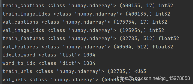
data = load_coco_data(pca_features=True)

# Print out all the keys and values from the data dictionary
for k, v in data.items():
    if type(v) == np.ndarray:
        print(k, type(v), v.shape, v.dtype)
    else:
        print(k, type(v), len(v))

查看数据

在使用数据集之前查看它的示例总是一个好主意。

您可以使用文件cs231n/coco_utils.py中的sample_coco_minibatch函数，从load_coco_data返回的数据结构中取样迷你批数据。运行以下命令对一小批训练数据进行采样，并显示图像及其说明。多次运行并查看结果有助于您了解数据集。

请注意，我们使用decode_captions函数对标题进行解码，并使用它们的Flickr URL动态下载图像，因此您必须连接到互联网才能查看图像。
ln[3]:

# Sample a minibatch and show the images and captions
batch_size = 3

captions, features, urls = sample_coco_minibatch(data, batch_size=batch_size)
for i, (caption, url) in enumerate(zip(captions, urls)):
    plt.imshow(image_from_url(url))
    plt.axis('off')
    caption_str = decode_captions(caption, data['idx_to_word'])
    plt.title(caption_str)
    plt.show()

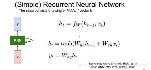
递归神经网络

正如在课堂上讨论的，我们将使用递归神经网络(RNN)语言模型来进行图像字幕。文件cs231n/rnn_layers.py包含递归神经网络所需的不同层类型的实现，文件cs231n/classifiers/rnn.py使用这些层来实现图像标题模型。

我们将首先在cs231n/rnn_layers.py中实现不同类型的RNN层。

注:长短期记忆(LSTM) RNN是普通RNN的一种变体。LSTM_Captioning.ipynb是可选的额外学分，所以现在不用担心cs231n/classifier/rnn.py和cs231n/rnn_layers.py中对LSTM的引用。

Vanilla RNN:step forward

打开文件cs231n/rnn_layers.py。这个文件实现了在递归神经网络中常用的不同类型的层的前向和后向传递。

首先实现函数rnn_step_forward，它实现了普通递归神经网络的单个时间步的前向传递。这样做之后，运行以下命令检查您的实现。您应该看到e-8或更小的错误。

def rnn_step_forward(x, prev_h, Wx, Wh, b):
    """Run the forward pass for a single timestep of a vanilla RNN using a tanh activation function.

    The input data has dimension D, the hidden state has dimension H,
    and the minibatch is of size N.

    Inputs:
    - x: Input data for this timestep, of shape (N, D)
    - prev_h: Hidden state from previous timestep, of shape (N, H)
    - Wx: Weight matrix for input-to-hidden connections, of shape (D, H)
    - Wh: Weight matrix for hidden-to-hidden connections, of shape (H, H)
    - b: Biases of shape (H,)

    Returns a tuple of:
    - next_h: Next hidden state, of shape (N, H)
    - cache: Tuple of values needed for the backward pass.
    """
    next_h, cache = None, None
    ##############################################################################
    # TODO: Implement a single forward step for the vanilla RNN. Store the next  #
    # hidden state and any values you need for the backward pass in the next_h   #
    # and cache variables respectively.                                          #
    ##############################################################################
    # *****START OF YOUR CODE (DO NOT DELETE/MODIFY THIS LINE)*****

    next_h = np.tanh(x.dot(Wx) + prev_h.dot(Wh) + b)
    cache = (x, prev_h, Wx, Wh, b, next_h)

    # *****END OF YOUR CODE (DO NOT DELETE/MODIFY THIS LINE)*****
    ##############################################################################
    #                               END OF YOUR CODE                             #
    ##############################################################################
    return next_h, cache

ln[4]:

N, D, H = 3, 10, 4

x = np.linspace(-0.4, 0.7, num=N*D).reshape(N, D)
prev_h = np.linspace(-0.2, 0.5, num=N*H).reshape(N, H)
Wx = np.linspace(-0.1, 0.9, num=D*H).reshape(D, H)
Wh = np.linspace(-0.3, 0.7, num=H*H).reshape(H, H)
b = np.linspace(-0.2, 0.4, num=H)

next_h, _ = rnn_step_forward(x, prev_h, Wx, Wh, b)
expected_next_h = np.asarray([
  [-0.58172089, -0.50182032, -0.41232771, -0.31410098],
  [ 0.66854692,  0.79562378,  0.87755553,  0.92795967],
  [ 0.97934501,  0.99144213,  0.99646691,  0.99854353]])

print('next_h error: ', rel_error(expected_next_h, next_h))

Vanilla RNN: step backward
在文件cs231n/rnn_layers.py中实现rnn_step_backward函数。这样做之后，运行下面的数字梯度检查您的实现。您应该看到e-8或更小的错误。

def rnn_step_backward(dnext_h, cache):
    """Backward pass for a single timestep of a vanilla RNN.

    Inputs:
    - dnext_h: Gradient of loss with respect to next hidden state, of shape (N, H)
    - cache: Cache object from the forward pass

    Returns a tuple of:
    - dx: Gradients of input data, of shape (N, D)
    - dprev_h: Gradients of previous hidden state, of shape (N, H)
    - dWx: Gradients of input-to-hidden weights, of shape (D, H)
    - dWh: Gradients of hidden-to-hidden weights, of shape (H, H)
    - db: Gradients of bias vector, of shape (H,)
    """
    dx, dprev_h, dWx, dWh, db = None, None, None, None, None
    ##############################################################################
    # TODO: Implement the backward pass for a single step of a vanilla RNN.      #
    #                                                                            #
    # HINT: For the tanh function, you can compute the local derivative in terms #
    # of the output value from tanh.                                             #
    ##############################################################################
    # *****START OF YOUR CODE (DO NOT DELETE/MODIFY THIS LINE)*****

    x, prev_h, Wx, Wh, b, tanh = cache
    dtanh = 1 - tanh ** 2  # [NxH]
    dnext_tanh = dnext_h * dtanh  # [NxH]
    dx = dnext_tanh.dot(Wx.T)  # [NxD]
    dprev_h = dnext_tanh.dot(Wh.T)  # [NxH]
    dWx = (x.T).dot(dnext_tanh)  # [DxH]
    dWh = (prev_h.T).dot(dnext_tanh)  # [DxH]
    db = dnext_tanh.sum(axis=0)  # [1xH]

    # *****END OF YOUR CODE (DO NOT DELETE/MODIFY THIS LINE)*****
    ##############################################################################
    #                               END OF YOUR CODE                             #
    ##############################################################################
    return dx, dprev_h, dWx, dWh, db

ln[5]:

from cs231n.rnn_layers import rnn_step_forward, rnn_step_backward
np.random.seed(231)
N, D, H = 4, 5, 6
x = np.random.randn(N, D)
h = np.random.randn(N, H)
Wx = np.random.randn(D, H)
Wh = np.random.randn(H, H)
b = np.random.randn(H)

out, cache = rnn_step_forward(x, h, Wx, Wh, b)

dnext_h = np.random.randn(*out.shape)

fx = lambda x: rnn_step_forward(x, h, Wx, Wh, b)[0]
fh = lambda prev_h: rnn_step_forward(x, h, Wx, Wh, b)[0]
fWx = lambda Wx: rnn_step_forward(x, h, Wx, Wh, b)[0]
fWh = lambda Wh: rnn_step_forward(x, h, Wx, Wh, b)[0]
fb = lambda b: rnn_step_forward(x, h, Wx, Wh, b)[0]

dx_num = eval_numerical_gradient_array(fx, x, dnext_h)
dprev_h_num = eval_numerical_gradient_array(fh, h, dnext_h)
dWx_num = eval_numerical_gradient_array(fWx, Wx, dnext_h)
dWh_num = eval_numerical_gradient_array(fWh, Wh, dnext_h)
db_num = eval_numerical_gradient_array(fb, b, dnext_h)

dx, dprev_h, dWx, dWh, db = rnn_step_backward(dnext_h, cache)

print('dx error: ', rel_error(dx_num, dx))
print('dprev_h error: ', rel_error(dprev_h_num, dprev_h))
print('dWx error: ', rel_error(dWx_num, dWx))
print('dWh error: ', rel_error(dWh_num, dWh))
print('db error: ', rel_error(db_num, db))

Vanilla RNN: forward
现在您已经实现了普通RNN的一个时间步的向前和向后传递，您将组合这些部分来实现处理整个数据序列的RNN。

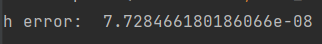
在cs231n/rnn_layers.py文件中，实现rnn_forward函数。这应该使用上面定义的rnn_step_forward函数来实现。这样做之后，运行以下命令检查您的实现。你应该看到e-7或更小的错误。

def rnn_forward(x, h0, Wx, Wh, b):
    """Run a vanilla RNN forward on an entire sequence of data.
    
    We assume an input sequence composed of T vectors, each of dimension D. The RNN uses a hidden
    size of H, and we work over a minibatch containing N sequences. After running the RNN forward,
    we return the hidden states for all timesteps.

    Inputs:
    - x: Input data for the entire timeseries, of shape (N, T, D)
    - h0: Initial hidden state, of shape (N, H)
    - Wx: Weight matrix for input-to-hidden connections, of shape (D, H)
    - Wh: Weight matrix for hidden-to-hidden connections, of shape (H, H)
    - b: Biases of shape (H,)

    Returns a tuple of:
    - h: Hidden states for the entire timeseries, of shape (N, T, H)
    - cache: Values needed in the backward pass
    """
    h, cache = None, None
    ##############################################################################
    # TODO: Implement forward pass for a vanilla RNN running on a sequence of    #
    # input data. You should use the rnn_step_forward function that you defined  #
    # above. You can use a for loop to help compute the forward pass.            #
    ##############################################################################
    # *****START OF YOUR CODE (DO NOT DELETE/MODIFY THIS LINE)*****

    N, T, D = x.shape
    H = h0.shape[1]
    prev_h = h0
    h = np.zeros((N, T, H))
    cache = []
    for i in range(T):
        prev_h, cache_h = rnn_step_forward(x[:, i, :], prev_h, Wx, Wh, b)
        h[:, i, :] = prev_h
        cache.append(cache_h)

    # *****END OF YOUR CODE (DO NOT DELETE/MODIFY THIS LINE)*****
    ##############################################################################
    #                               END OF YOUR CODE                             #
    ##############################################################################
    return h, cache

ln[6]:

N, T, D, H = 2, 3, 4, 5

x = np.linspace(-0.1, 0.3, num=N*T*D).reshape(N, T, D)
h0 = np.linspace(-0.3, 0.1, num=N*H).reshape(N, H)
Wx = np.linspace(-0.2, 0.4, num=D*H).reshape(D, H)
Wh = np.linspace(-0.4, 0.1, num=H*H).reshape(H, H)
b = np.linspace(-0.7, 0.1, num=H)

h, _ = rnn_forward(x, h0, Wx, Wh, b)
expected_h = np.asarray([
  [
    [-0.42070749, -0.27279261, -0.11074945,  0.05740409,  0.22236251],
    [-0.39525808, -0.22554661, -0.0409454,   0.14649412,  0.32397316],
    [-0.42305111, -0.24223728, -0.04287027,  0.15997045,  0.35014525],
  ],
  [
    [-0.55857474, -0.39065825, -0.19198182,  0.02378408,  0.23735671],
    [-0.27150199, -0.07088804,  0.13562939,  0.33099728,  0.50158768],
    [-0.51014825, -0.30524429, -0.06755202,  0.17806392,  0.40333043]]])
print('h error: ', rel_error(expected_h, h))

Vanilla RNN: backward

def rnn_backward(dh, cache):
    """Compute the backward pass for a vanilla RNN over an entire sequence of data.

    Inputs:
    - dh: Upstream gradients of all hidden states, of shape (N, T, H)
    
    NOTE: 'dh' contains the upstream gradients produced by the 
    individual loss functions at each timestep, *not* the gradients
    being passed between timesteps (which you'll have to compute yourself
    by calling rnn_step_backward in a loop).

    Returns a tuple of:
    - dx: Gradient of inputs, of shape (N, T, D)
    - dh0: Gradient of initial hidden state, of shape (N, H)
    - dWx: Gradient of input-to-hidden weights, of shape (D, H)
    - dWh: Gradient of hidden-to-hidden weights, of shape (H, H)
    - db: Gradient of biases, of shape (H,)
    """
    dx, dh0, dWx, dWh, db = None, None, None, None, None
    ##############################################################################
    # TODO: Implement the backward pass for a vanilla RNN running an entire      #
    # sequence of data. You should use the rnn_step_backward function that you   #
    # defined above. You can use a for loop to help compute the backward pass.   #
    ##############################################################################
    # *****START OF YOUR CODE (DO NOT DELETE/MODIFY THIS LINE)*****

    N, T, H = dh.shape
    dxl, dprev_h, dWx, dWh, db = rnn_step_backward(dh[:, T - 1, :], cache[T - 1])
    D = dxl.shape[1]
    dx = np.zeros((N, T, D))
    dx[:, T - 1, :] = dxl
    for i in range(T - 2, -1, -1):
        dxc, dprev_hc, dWxc, dWhc, dbc = rnn_step_backward(dh[:, i, :] + dprev_h, cache[i])
        dx[:, i, :] += dxc
        dprev_h = dprev_hc
        dWx += dWxc
        dWh += dWhc
        db += dbc
    dh0 = dprev_h

    # *****END OF YOUR CODE (DO NOT DELETE/MODIFY THIS LINE)*****
    ##############################################################################
    #                               END OF YOUR CODE                             #
    ##############################################################################
    return dx, dh0, dWx, dWh, db

ln[7]:

np.random.seed(231)

N, D, T, H = 2, 3, 10, 5

x = np.random.randn(N, T, D)
h0 = np.random.randn(N, H)
Wx = np.random.randn(D, H)
Wh = np.random.randn(H, H)
b = np.random.randn(H)

out, cache = rnn_forward(x, h0, Wx, Wh, b)

dout = np.random.randn(*out.shape)

dx, dh0, dWx, dWh, db = rnn_backward(dout, cache)

fx = lambda x: rnn_forward(x, h0, Wx, Wh, b)[0]
fh0 = lambda h0: rnn_forward(x, h0, Wx, Wh, b)[0]
fWx = lambda Wx: rnn_forward(x, h0, Wx, Wh, b)[0]
fWh = lambda Wh: rnn_forward(x, h0, Wx, Wh, b)[0]
fb = lambda b: rnn_forward(x, h0, Wx, Wh, b)[0]

dx_num = eval_numerical_gradient_array(fx, x, dout)
dh0_num = eval_numerical_gradient_array(fh0, h0, dout)
dWx_num = eval_numerical_gradient_array(fWx, Wx, dout)
dWh_num = eval_numerical_gradient_array(fWh, Wh, dout)
db_num = eval_numerical_gradient_array(fb, b, dout)

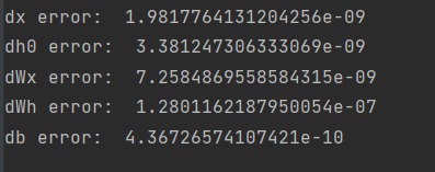
print('dx error: ', rel_error(dx_num, dx))
print('dh0 error: ', rel_error(dh0_num, dh0))
print('dWx error: ', rel_error(dWx_num, dWx))
print('dWh error: ', rel_error(dWh_num, dWh))
print('db error: ', rel_error(db_num, db))

Word embedding: forward
在深度学习系统中，我们通常使用向量来表示单词。词汇表中的每个单词都将与一个向量相关联，这些向量将与系统的其余部分联合学习。

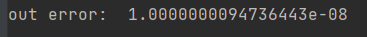
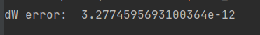
在文件cs231n/rnn_layers.py中，实现函数word_embeddding_forward来将单词(由整数表示)转换为向量。运行以下命令检查您的实现。您应该看到一个e-8或更小的错误。

def word_embedding_forward(x, W):
    """Forward pass for word embeddings.
    
    We operate on minibatches of size N where
    each sequence has length T. We assume a vocabulary of V words, assigning each
    word to a vector of dimension D.

    Inputs:
    - x: Integer array of shape (N, T) giving indices of words. Each element idx
      of x muxt be in the range 0 <= idx < V.
    - W: Weight matrix of shape (V, D) giving word vectors for all words.

    Returns a tuple of:
    - out: Array of shape (N, T, D) giving word vectors for all input words.
    - cache: Values needed for the backward pass
    """
    out, cache = None, None
    ##############################################################################
    # TODO: Implement the forward pass for word embeddings.                      #
    #                                                                            #
    # HINT: This can be done in one line using NumPy's array indexing.           #
    ##############################################################################
    # *****START OF YOUR CODE (DO NOT DELETE/MODIFY THIS LINE)*****

    out = W[x]
    cache = (x, W)

    # *****END OF YOUR CODE (DO NOT DELETE/MODIFY THIS LINE)*****
    ##############################################################################
    #                               END OF YOUR CODE                             #
    ##############################################################################
    return out, cache

ln[8]:


N, T, V, D = 2, 4, 5, 3

x = np.asarray([[0, 3, 1, 2], [2, 1, 0, 3]])
W = np.linspace(0, 1, num=V*D).reshape(V, D)

out, _ = word_embedding_forward(x, W)
expected_out = np.asarray([
 [[ 0.,          0.07142857,  0.14285714],
  [ 0.64285714,  0.71428571,  0.78571429],
  [ 0.21428571,  0.28571429,  0.35714286],
  [ 0.42857143,  0.5,         0.57142857]],
 [[ 0.42857143,  0.5,         0.57142857],
  [ 0.21428571,  0.28571429,  0.35714286],
  [ 0.,          0.07142857,  0.14285714],
  [ 0.64285714,  0.71428571,  0.78571429]]])

print('out error: ', rel_error(expected_out, out))

Word embedding: backward

def word_embedding_backward(dout, cache):
    """Backward pass for word embeddings.
    
    We cannot back-propagate into the words
    since they are integers, so we only return gradient for the word embedding
    matrix.

    HINT: Look up the function np.add.at

    Inputs:
    - dout: Upstream gradients of shape (N, T, D)
    - cache: Values from the forward pass

    Returns:
    - dW: Gradient of word embedding matrix, of shape (V, D)
    """
    dW = None
    ##############################################################################
    # TODO: Implement the backward pass for word embeddings.                     #
    #                                                                            #
    # Note that words can appear more than once in a sequence.                   #
    # HINT: Look up the function np.add.at                                       #
    ##############################################################################
    # *****START OF YOUR CODE (DO NOT DELETE/MODIFY THIS LINE)*****

    x, W = cache
    dW = np.zeros(W.shape)
    np.add.at(dW, x, dout)

    # *****END OF YOUR CODE (DO NOT DELETE/MODIFY THIS LINE)*****
    ##############################################################################
    #                               END OF YOUR CODE                             #
    ##############################################################################
    return dW

ln[9]:

np.random.seed(231)

N, T, V, D = 50, 3, 5, 6
x = np.random.randint(V, size=(N, T))
W = np.random.randn(V, D)

out, cache = word_embedding_forward(x, W)
dout = np.random.randn(*out.shape)
dW = word_embedding_backward(dout, cache)

f = lambda W: word_embedding_forward(x, W)[0]
dW_num = eval_numerical_gradient_array(f, W, dout)

print('dW error: ', rel_error(dW, dW_num))

Temporal Affine layer
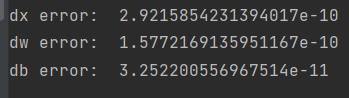
在每个时间步上，我们使用一个仿射函数将该时间步上的RNN隐向量转换为词汇表中每个单词的分数。因为这与赋值2中实现的仿射层非常相似，所以我们在cs231n/rnn_layers.py文件中的temporal_affine_forward和temporal_affine_backward函数中为您提供了这个函数。运行以下命令对实现执行数值梯度检查。你应该看到e-9或更小的错误。

ln[10]:

np.random.seed(231)

# Gradient check for temporal affine layer
N, T, D, M = 2, 3, 4, 5
x = np.random.randn(N, T, D)
w = np.random.randn(D, M)
b = np.random.randn(M)

out, cache = temporal_affine_forward(x, w, b)

dout = np.random.randn(*out.shape)

fx = lambda x: temporal_affine_forward(x, w, b)[0]
fw = lambda w: temporal_affine_forward(x, w, b)[0]
fb = lambda b: temporal_affine_forward(x, w, b)[0]

dx_num = eval_numerical_gradient_array(fx, x, dout)
dw_num = eval_numerical_gradient_array(fw, w, dout)
db_num = eval_numerical_gradient_array(fb, b, dout)

dx, dw, db = temporal_affine_backward(dout, cache)

print('dx error: ', rel_error(dx_num, dx))
print('dw error: ', rel_error(dw_num, dw))
print('db error: ', rel_error(db_num, db))

Temporal Softmax loss
在RNN语言模型中，我们在每个时间步骤中为词汇表中的每个单词生成一个分数。我们知道每个时间步的地面真实值，因此我们使用softmax损失函数来计算每个时间步的损失和梯度。我们将随着时间的推移的损失相加，并在小批量中平均它们。

但是有一个问题:因为我们操作的是小批量，不同的标题可能有不同的长度，所以我们在每个标题的末尾添加标记，这样它们都有相同的长度。我们不想让这些标记计入损失或梯度，因此除了分数和地面真值标签外，我们的损失函数还接受一个掩码数组，告诉它分数的哪些元素计入损失。

因为这非常类似于您在分配1中实现的softmax损失函数，我们已经为您实现了这个损失函数;查看cs231n/rnn_layers.py文件中的temporal_softmax_loss函数。

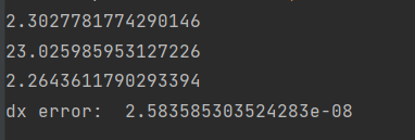
运行以下单元格以检查损失，并对函数执行数值梯度检查。你应该看到dx的错误，其数量级是e-7或更小。
ln[11]:

# Sanity check for temporal softmax loss
from cs231n.rnn_layers import temporal_softmax_loss

N, T, V = 100, 1, 10

def check_loss(N, T, V, p):
    x = 0.001 * np.random.randn(N, T, V)
    y = np.random.randint(V, size=(N, T))
    mask = np.random.rand(N, T) <= p
    print(temporal_softmax_loss(x, y, mask)[0])
  
check_loss(100, 1, 10, 1.0)   # Should be about 2.3
check_loss(100, 10, 10, 1.0)  # Should be about 23
check_loss(5000, 10, 10, 0.1) # Should be about 2.3

# Gradient check for temporal softmax loss
N, T, V = 7, 8, 9

x = np.random.randn(N, T, V)
y = np.random.randint(V, size=(N, T))
mask = (np.random.rand(N, T) > 0.5)

loss, dx = temporal_softmax_loss(x, y, mask, verbose=False)

dx_num = eval_numerical_gradient(lambda x: temporal_softmax_loss(x, y, mask)[0], x, verbose=False)

print('dx error: ', rel_error(dx, dx_num))

RNN for image captioning
现在已经实现了必要的层，可以将它们组合起来构建图像标题模型。打开文件cs231n/classifier /rnn.py，查看CaptioningRNN类。

在损失函数中实现模型的前向和后向传递。现在你只需要实现cell_type='rnn’的情况;稍后您将实现LSTM用例。这样做之后，运行下面的程序，使用一个小的测试用例检查您的前向传递;你应该看到e-10或更小的错误。

############################################################################
        # TODO: Implement the forward and backward passes for the CaptioningRNN.   #
        # In the forward pass you will need to do the following:                   #
        # (1) Use an affine transformation to compute the initial hidden state     #
        #     from the image features. This should produce an array of shape (N, H)#
        # (2) Use a word embedding layer to transform the words in captions_in     #
        #     from indices to vectors, giving an array of shape (N, T, W).         #
        # (3) Use either a vanilla RNN or LSTM (depending on self.cell_type) to    #
        #     process the sequence of input word vectors and produce hidden state  #
        #     vectors for all timesteps, producing an array of shape (N, T, H).    #
        # (4) Use a (temporal) affine transformation to compute scores over the    #
        #     vocabulary at every timestep using the hidden states, giving an      #
        #     array of shape (N, T, V).                                            #
        # (5) Use (temporal) softmax to compute loss using captions_out, ignoring  #
        #     the points where the output word is <NULL> using the mask above.     #
        #                                                                          #
        #                                                                          #
        # Do not worry about regularizing the weights or their gradients!          #
        #                                                                          #
        # In the backward pass you will need to compute the gradient of the loss   #
        # with respect to all model parameters. Use the loss and grads variables   #
        # defined above to store loss and gradients; grads[k] should give the      #
        # gradients for self.params[k].                                            #
        #                                                                          #
        # Note also that you are allowed to make use of functions from layers.py   #
        # in your implementation, if needed.                                       #
        ############################################################################
        # *****START OF YOUR CODE (DO NOT DELETE/MODIFY THIS LINE)*****

        h0 = features.dot(W_proj) + b_proj  # [NxH]
        x, cache_we = word_embedding_forward(captions_in, W_embed)  # [NxTxW]
        if self.cell_type == 'rnn':
            h, cache_rnn = rnn_forward(x, h0, Wx, Wh, b)  # [NxTxH]
        else:
            h, cache_lstm = lstm_forward(x, h0, Wx, Wh, b)  # [NxTxH]
        out, cache_voc = temporal_affine_forward(h, W_vocab, b_vocab)  # [NxTxV]
        loss, dout = temporal_softmax_loss(out, captions_out, mask, verbose=False)

        # gradients
        dh, dW_vocab, db_vocab = temporal_affine_backward(dout, cache_voc)
        if self.cell_type == 'rnn':
            dx, dh0, dWx, dWh, db = rnn_backward(dh, cache_rnn)
        else:
            dx, dh0, dWx, dWh, db = lstm_backward(dh, cache_lstm)
        dW_embed = word_embedding_backward(dx, cache_we)
        dW_proj = features.T.dot(dh0)
        db_proj = dh0.sum(axis=0)
        grads = {'W_vocab': dW_vocab, 'b_vocab': db_vocab, 'Wx': dWx, 'Wh': dWh,
                 'b': db, 'W_embed': dW_embed, 'W_proj': dW_proj, 'b_proj': db_proj}

        # *****END OF YOUR CODE (DO NOT DELETE/MODIFY THIS LINE)*****
        ############################################################################
        #                             END OF YOUR CODE                             #
        ############################################################################

ln[12]:

N, D, W, H = 10, 20, 30, 40
word_to_idx = {'<NULL>': 0, 'cat': 2, 'dog': 3}
V = len(word_to_idx)
T = 13

model = CaptioningRNN(word_to_idx,
          input_dim=D,
          wordvec_dim=W,
          hidden_dim=H,
          cell_type='rnn',
          dtype=np.float64)

# Set all model parameters to fixed values
for k, v in model.params.items():
    model.params[k] = np.linspace(-1.4, 1.3, num=v.size).reshape(*v.shape)

features = np.linspace(-1.5, 0.3, num=(N * D)).reshape(N, D)
captions = (np.arange(N * T) % V).reshape(N, T)

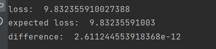
loss, grads = model.loss(features, captions)
expected_loss = 9.83235591003

print('loss: ', loss)
print('expected loss: ', expected_loss)
print('difference: ', abs(loss - expected_loss))

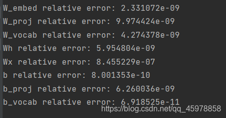
梯度检查：
ln[13]:

np.random.seed(231)

batch_size = 2
timesteps = 3
input_dim = 4
wordvec_dim = 5
hidden_dim = 6
word_to_idx = {'<NULL>': 0, 'cat': 2, 'dog': 3}
vocab_size = len(word_to_idx)

captions = np.random.randint(vocab_size, size=(batch_size, timesteps))
features = np.random.randn(batch_size, input_dim)

model = CaptioningRNN(word_to_idx,
          input_dim=input_dim,
          wordvec_dim=wordvec_dim,
          hidden_dim=hidden_dim,
          cell_type='rnn',
          dtype=np.float64,
        )

loss, grads = model.loss(features, captions)

for param_name in sorted(grads):
    f = lambda _: model.loss(features, captions)[0]
    param_grad_num = eval_numerical_gradient(f, model.params[param_name], verbose=False, h=1e-6)
    e = rel_error(param_grad_num, grads[param_name])
    print('%s relative error: %e' % (param_name, e))

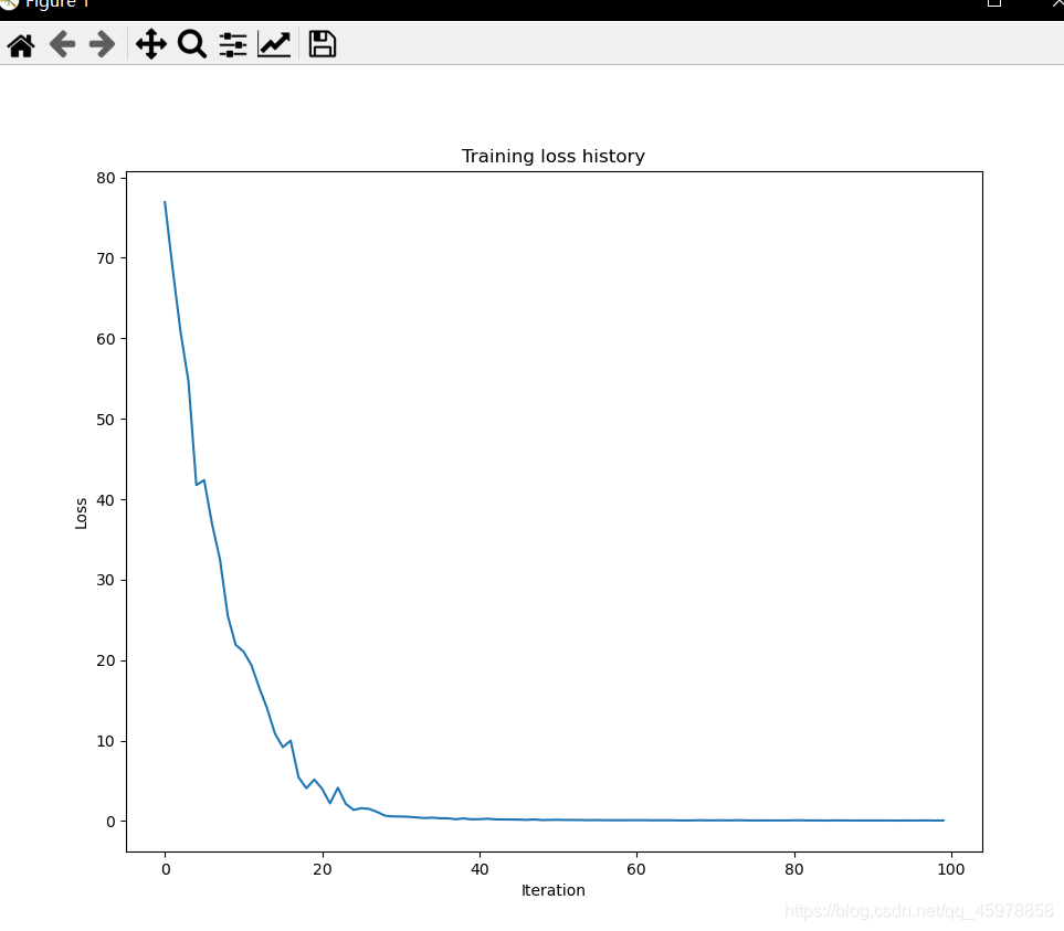
Overfit小的数据

与我们在之前的作业中用来训练图像分类模型的Solver类类似，在这次作业中，我们使用了一个CaptioningSolver类来训练图像标题模型。打开文件cs231n/captioning_solver.py，通读CaptioningSolver类;看起来应该很眼熟。

一旦您熟悉了API，就运行下面的程序，以确保您的模型超过了100个训练示例的小样本。你应该看到最终损失小于0.1。
ln[14]:

np.random.seed(231)

small_data = load_coco_data(max_train=50)

small_rnn_model = CaptioningRNN(
          cell_type='rnn',
          word_to_idx=data['word_to_idx'],
          input_dim=data['train_features'].shape[1],
          hidden_dim=512,
          wordvec_dim=256,
        )

small_rnn_solver = CaptioningSolver(small_rnn_model, small_data,
           update_rule='adam',
           num_epochs=50,
           batch_size=25,
           optim_config={
             'learning_rate': 5e-3,
           },
           lr_decay=0.95,
           verbose=True, print_every=10,
         )

small_rnn_solver.train()

# Plot the training losses
plt.plot(small_rnn_solver.loss_history)
plt.xlabel('Iteration')
plt.ylabel('Loss')
plt.title('Training loss history')
plt.show()

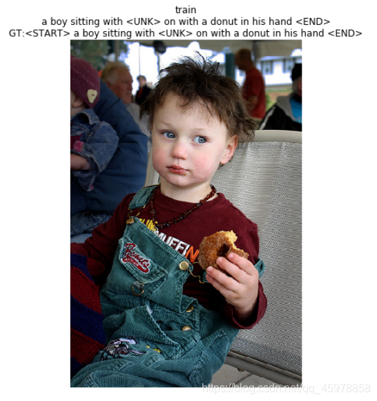
Test-time sampling

与分类模型不同，图像标题模型在训练时和测试时的行为非常不同。在训练时，我们可以访问ground-truth标题，因此我们在每个时间步向RNN输入ground-truth单词。在测试时，我们从每个时间步上的词汇分布中抽取样本，并在下一个时间步上将样本作为输入输入RNN。

在文件cs231n/classifier/rnn.py中，实现测试时间采样的示例方法。这样做之后，运行以下操作，从过度拟合的模型中对训练和验证数据进行取样。训练数据上的样本应该很好;验证数据上的示例可能没有意义。

    def sample(self, features, max_length=30):
        """
        Run a test-time forward pass for the model, sampling captions for input
        feature vectors.

        At each timestep, we embed the current word, pass it and the previous hidden
        state to the RNN to get the next hidden state, use the hidden state to get
        scores for all vocab words, and choose the word with the highest score as
        the next word. The initial hidden state is computed by applying an affine
        transform to the input image features, and the initial word is the <START>
        token.

        For LSTMs you will also have to keep track of the cell state; in that case
        the initial cell state should be zero.

        Inputs:
        - features: Array of input image features of shape (N, D).
        - max_length: Maximum length T of generated captions.

        Returns:
        - captions: Array of shape (N, max_length) giving sampled captions,
          where each element is an integer in the range [0, V). The first element
          of captions should be the first sampled word, not the <START> token.
        """
        N = features.shape[0]
        captions = self._null * np.ones((N, max_length), dtype=np.int32)

        # Unpack parameters
        W_proj, b_proj = self.params["W_proj"], self.params["b_proj"]
        W_embed = self.params["W_embed"]
        Wx, Wh, b = self.params["Wx"], self.params["Wh"], self.params["b"]
        W_vocab, b_vocab = self.params["W_vocab"], self.params["b_vocab"]

        ###########################################################################
        # TODO: Implement test-time sampling for the model. You will need to      #
        # initialize the hidden state of the RNN by applying the learned affine   #
        # transform to the input image features. The first word that you feed to  #
        # the RNN should be the <START> token; its value is stored in the         #
        # variable self._start. At each timestep you will need to do to:          #
        # (1) Embed the previous word using the learned word embeddings           #
        # (2) Make an RNN step using the previous hidden state and the embedded   #
        #     current word to get the next hidden state.                          #
        # (3) Apply the learned affine transformation to the next hidden state to #
        #     get scores for all words in the vocabulary                          #
        # (4) Select the word with the highest score as the next word, writing it #
        #     (the word index) to the appropriate slot in the captions variable   #
        #                                                                         #
        # For simplicity, you do not need to stop generating after an <END> token #
        # is sampled, but you can if you want to.                                 #
        #                                                                         #
        # HINT: You will not be able to use the rnn_forward or lstm_forward       #
        # functions; you'll need to call rnn_step_forward or lstm_step_forward in #
        # a loop.                                                                 #
        #                                                                         #
        # NOTE: we are still working over minibatches in this function. Also if   #
        # you are using an LSTM, initialize the first cell state to zeros.        #
        ###########################################################################
        # *****START OF YOUR CODE (DO NOT DELETE/MODIFY THIS LINE)*****

        h0 = features.dot(W_proj) + b_proj
        c0 = np.zeros(h0.shape)
        V, W = W_embed.shape
        x = np.ones((N, W)) * W_embed[self._start]
        for i in range(max_length):
            if self.cell_type == 'rnn':
                next_h, _ = rnn_step_forward(x, h0, Wx, Wh, b)
            else:
                next_h, next_c, _ = lstm_step_forward(x, h0, c0, Wx, Wh, b)
                c0 = next_c
            out = next_h.dot(W_vocab) + b_vocab
            max_indices = out.argmax(axis=1)
            captions[:, i] = max_indices
            x = W_embed[max_indices]
            h0 = next_h

        # *****END OF YOUR CODE (DO NOT DELETE/MODIFY THIS LINE)*****
        ############################################################################
        #                             END OF YOUR CODE                             #
        ############################################################################
        return captions

ln[15]:

for split in ['train', 'val']:
    minibatch = sample_coco_minibatch(small_data, split=split, batch_size=2)
    gt_captions, features, urls = minibatch
    gt_captions = decode_captions(gt_captions, data['idx_to_word'])

    sample_captions = small_rnn_model.sample(features)
    sample_captions = decode_captions(sample_captions, data['idx_to_word'])

    for gt_caption, sample_caption, url in zip(gt_captions, sample_captions, urls):
        plt.imshow(image_from_url(url))
        plt.title('%s\n%s\nGT:%s' % (split, sample_caption, gt_caption))
        plt.axis('off')
        plt.show()

内联问题1
在我们当前的图像字幕设置中，RNN语言模型在每个时间步产生一个单词作为输出。然而，提出这个问题的另一种方法是训练网络操作字符(例如’a’， 'b’等)而不是单词，因此在它的每一个时间步，它接收前一个字符作为输入，并试图预测序列中的下一个字符。例如，网络可能生成如下的标题
‘A’, ’ ', ‘c’, ‘a’, ‘t’, ’ ', ‘o’, ‘n’, ’ ', ‘a’, ’ ', ‘b’, ‘e’, ‘d’
你能描述一下使用字符级RNN的图像字幕模型的一个优点吗?你还能描述一个缺点吗?提示:有几个有效的答案，但是比较字级模型和字符级模型的参数空间可能是有用的。
回答
使用字符级RNN的图像字幕模型的一个优点是它们的词汇量非常小。例如，假设我们有一个包含100万个不同单词的数据集。如果我们使用单词级模型，那么它将比字符级模型需要更多的内存，因为用于表示所有单词的字符数量将更小。
一个缺点是参数的数量会增加，因为我们有一个更大的序列。在前面的例子中，隐藏层的数量将等于字符的数量(不考虑空格字符的10层)。另一方面，使用字层模型，隐藏层的数量将等于5。拥有少量的参数在计算上更有效，更不容易消失/爆炸梯度。

Esaka7

关注

1
点赞
踩
4

收藏

觉得还不错? 一键收藏
打赏
0
评论
CS231n-assignment3-Image Captioning with RNNs

在这个练习中，您将实现一个vanilla递归神经网络，并使用它们来训练一个模型，可以为图像生成新的标题。ln[1]:# As usual, a bit of setupimport time, os, jsonimport numpy as npimport matplotlib.pyplot as pltfrom cs231n.gradient_check import eval_numerical_gradient, eval_numerical_gradient_arrayfrom c
复制链接

扫一扫