tensorboard使用界面介绍以及使用方法（看这篇就够了，都有源码可以直接测试）

最新推荐文章于 2024-06-12 11:24:25 发布

ERROR_LESS

最新推荐文章于 2024-06-12 11:24:25 发布

阅读量3k

点赞数 4

分类专栏： tensorflow python 文章标签： tensorflow python 人工智能

本文链接：https://blog.csdn.net/qq_47058489/article/details/125780106

版权

python 同时被 2 个专栏收录

19 篇文章 0 订阅

订阅专栏

tensorflow

3 篇文章 0 订阅

订阅专栏

0 总述

简要概述所显示的仪表板（顶部导航栏中的选项卡）：

Scalars显示损失和准确率指标在每个时期如何变化。您还可以使用它来跟踪训练速度，学习率和其他标量值。
Graphs 可帮助您可视化模型。在这种情况下，将显示层的Keras图，这可以帮助您确保正确构建。
Distributions 和 Histograms 显示张量随时间的分布。这对于可视化权重和偏差并验证它们是否以预期的方式变化很有用。

1 Scalars：记录训练过程中各标量的变化

1.1 概述

参考文档

机器学习总是涉及理解关键指标，例如损失 (loss) ，以及它们如何随着训练的进行而变化。例如，这些指标可以帮助您了解模型是否过拟合，或者是否不必要地训练了太长时间。您可能需要比较不同训练中的这些指标，以帮助调试和改善模型。

1.2 代码样例

在代码的注释中有详细解释各部分流程：

#!/usr/bin/env python
# -*- coding: utf-8 -*-
# @Time : 2022/7/14 11:10
# @Author : hqc
# @File : scalars_usage.py
# @Software: PyCharm

### import necessary modules

import tensorflow as tf
from tensorflow import keras
import datetime

import numpy as np
print("TensorFlow version: ", tf.__version__)

### set data to training regression

data_size = 1000
# 80% of the data is for training.
train_pct = 0.8
train_size = int(data_size * train_pct)

# Create some input data between -1 and 1 and randomize it.
x = np.linspace(-1, 1, data_size) # create 1000 number between (-1, 1) evenly
np.random.shuffle(x)

# Generate the output data.
# y = 0.5x + 2 + noise
# noise is created by a normal distribution with mean-value of 0 and standard deviation of 0.05
# shape of '(data_size, )' means one-dimensional array with 1000 elements
y = 0.5 * x + 2 + np.random.normal(0, 0.05, (data_size, ))

# Split into test and train pairs.
x_train, y_train = x[:train_size], y[:train_size] # the top 800 figures
x_test, y_test = x[train_size:], y[train_size:] # the last 200 figures

### Training the model and logging loss

# set the log directory and define a tensorboard callback
logdir = "logs/scalars/" + datetime.datetime.now().strftime("%Y%m%d-%H%M%S")
tensorboard_callback = keras.callbacks.TensorBoard(log_dir=logdir)

# create a model with 2 dense layer
model = keras.models.Sequential([
    keras.layers.Dense(16, input_dim=1),
    keras.layers.Dense(1),
])
# compile the model
model.compile(
    loss='mse', # keras.losses.mean_squared_error
    optimizer=keras.optimizers.SGD(learning_rate=0.2),
)
print("Training ... With default parameters, this takes less than 10 seconds.")

# training
training_history = model.fit(
    x_train, # input
    y_train, # output
    batch_size=train_size,
    verbose=0, # Suppress chatty output; use Tensorboard instead
    epochs=100,
    validation_data=(x_test, y_test),
    callbacks=[tensorboard_callback],
)
print("Average test loss: ", np.average(training_history.history['loss']))

1.3 运行查看

命令行中输入：PS D:\research\python learning\tensorflow learning> tensorboard --logdir tensorboard/logs/scalars

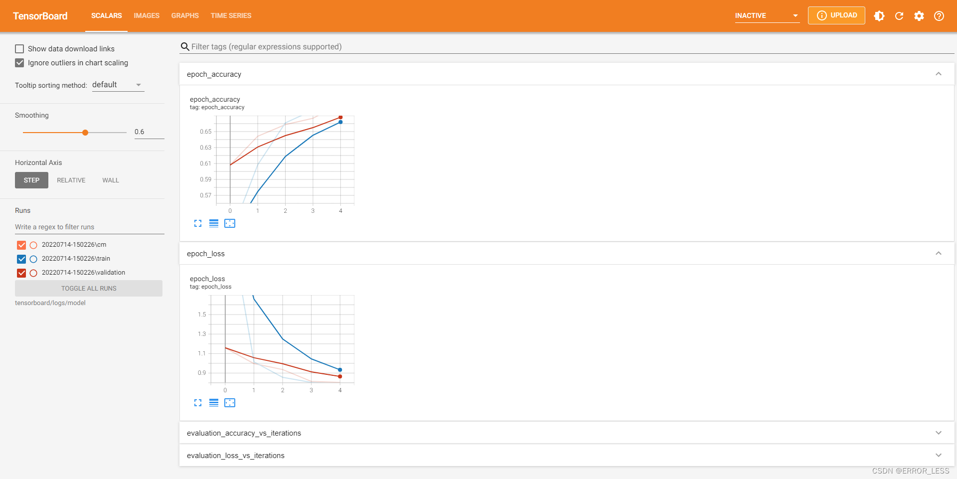
可查看到页面：
在这里插入图片描述
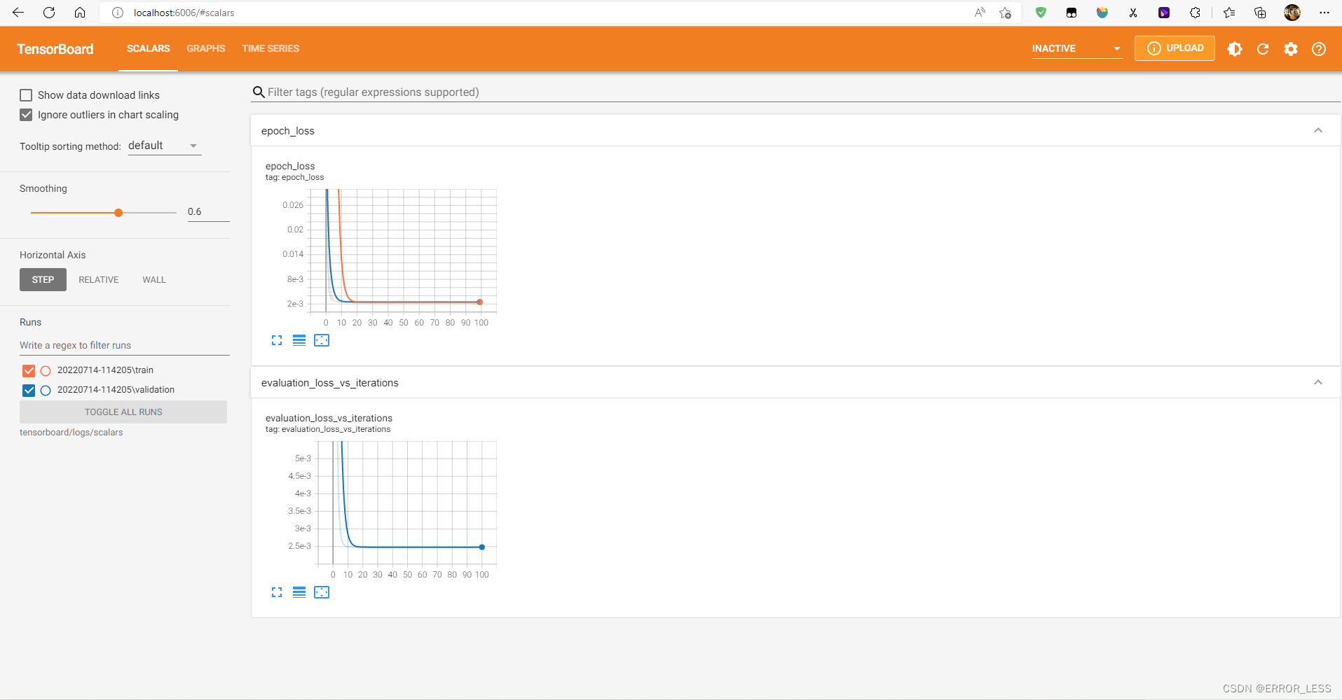
可见，对于训练和验证，损失都在持续降低，最后慢慢稳定下来，这意味着这个模型的指标非常好！

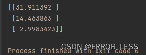
1.4 实际验证

给定 (60, 25, 2), 方程式 y = 0.5x + 2 应该会输出 (32, 14.5, 3). 模型会输出一样的结果吗?
加入以下代码：

### predict a real data
print(model.predict([60, 25, 2]))
# 理想的输出结果是:
# [[32.0]
#  [14.5]
#  [ 3.0]]

输出结果如下：可见很符合！
在这里插入图片描述

1.5 高阶应用：记录自定义的标量

重新训练回归模型并记录自定义学习率。如以下步骤所示：

使用 tf.summary.create_file_writer() 创建文件编写器。
定义自定义学习率函数。这将传递给 Keras LearningRateScheduler 回调。
在学习率函数内部，使用 tf.summary.scalar() 记录自定义学习率。
将 LearningRateScheduler 回调传递给 Model.fit()。

完整代码：

#!/usr/bin/env python
# -*- coding: utf-8 -*-
# @Time : 2022/7/14 11:10
# @Author : hqc
# @File : scalars_usage.py
# @Software: PyCharm

### import necessary modules

import tensorflow as tf
from tensorflow import keras
import datetime

import numpy as np
print("TensorFlow version: ", tf.__version__)

### set data to training regression

data_size = 1000
# 80% of the data is for training.
train_pct = 0.8
train_size = int(data_size * train_pct)

# Create some input data between -1 and 1 and randomize it.
x = np.linspace(-1, 1, data_size) # create 1000 number between (-1, 1) evenly
np.random.shuffle(x)

# Generate the output data.
# y = 0.5x + 2 + noise
# noise is created by a normal distribution with mean-value of 0 and standard deviation of 0.05
# shape of '(data_size, )' means one-dimensional array with 1000 elements
y = 0.5 * x + 2 + np.random.normal(0, 0.05, (data_size, ))

# Split into test and train pairs.
x_train, y_train = x[:train_size], y[:train_size] # the top 800 figures
x_test, y_test = x[train_size:], y[train_size:] # the last 200 figures



### set the log directory and define a tensorboard callback
logdir = "logs/scalars/" + datetime.datetime.now().strftime("%Y%m%d-%H%M%S")
tensorboard_callback = keras.callbacks.TensorBoard(log_dir=logdir)

### log custom scalars
# create a writer
file_writer = tf.summary.create_file_writer(logdir + "/metrics")
file_writer.set_as_default() # when migrate tf1 to tf2, this is useful

# define a learning_rate fn
def lr_schedule(epoch):
  """
  Returns a custom learning rate that decreases as epochs progress.
  """
  learning_rate = 0.2
  if epoch > 10:
    learning_rate = 0.02
  if epoch > 20:
    learning_rate = 0.01
  if epoch > 50:
    learning_rate = 0.005

  tf.summary.scalar('learning rate', data=learning_rate, step=epoch) # used to log it
  return learning_rate

# define a lr callback
lr_callback = keras.callbacks.LearningRateScheduler(lr_schedule)

### create a model with 2 dense layer
model = keras.models.Sequential([
    keras.layers.Dense(16, input_dim=1),
    keras.layers.Dense(1),
])
### compile the model
model.compile(
    loss='mse', # keras.losses.mean_squared_error
    optimizer=keras.optimizers.SGD(learning_rate=0.2),
)
print("Training ... With default parameters, this takes less than 10 seconds.")

### training
training_history = model.fit(
    x_train, # input
    y_train, # output
    batch_size=train_size,
    verbose=0, # Suppress chatty output; use Tensorboard instead
    epochs=100,
    validation_data=(x_test, y_test),
    callbacks=[tensorboard_callback, lr_callback],
)
print("Average test loss: ", np.average(training_history.history['loss']))

### predict a real data
print(model.predict([60, 25, 2]))
# 理想的输出结果是:
# [[32.0]
#  [14.5]
#  [ 3.0]]

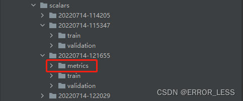
运行后发现：log里边多了一个metrics文件夹，这就是保存自定义学习率的地方
在这里插入图片描述
运行结果查看：

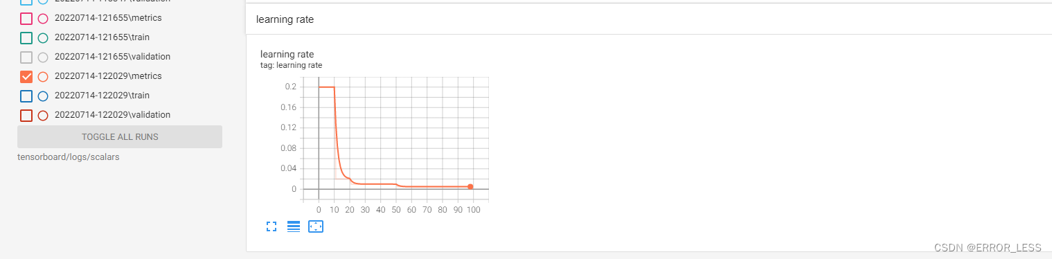
可见可以查看到学习率的训练过程变化~

2 Image：显示图像数据

2.1 概述

参考文档

使用 TensorFlow Image Summary API，您可以轻松地在 TensorBoard 中记录张量和任意图像并进行查看。这在采样和检查输入数据，或可视化层权重和生成的张量方面非常实用。您还可以将诊断数据记录为图像，这在模型开发过程中可能会有所帮助。

在本教程中，您将了解如何使用 Image Summary API 将张量可视化为图像。您还将了解如何获取任意图像，将其转换为张量并在 TensorBoard 中进行可视化。教程将通过一个简单而真实的示例，向您展示使用图像摘要了解模型性能。

2.2 可视化一张图片代码样例

#!/usr/bin/env python
# -*- coding: utf-8 -*-
# @Time : 2022/7/14 12:40
# @Author : hqc
# @File : image_usage.py
# @Software: PyCharm

### import necessary modules

from datetime import datetime
import io # related to file reading and writing
import itertools # used to operate the iterator
#from packaging import version # 语义化版本
#from six.moves import range # six is used to compatible with py2 and py3

import tensorflow as tf
from tensorflow import keras

import matplotlib.pyplot as plt
import numpy as np
import sklearn.metrics # 评价指标

print("TensorFlow version: ", tf.__version__)

### download Fashion-MNIST dataset
# Download the data. The data is already divided into train and test.
# The labels are integers representing classes.
fashion_mnist = keras.datasets.fashion_mnist
(train_images, train_labels), (test_images, test_labels) = \
    fashion_mnist.load_data()

# Names of the integer classes, i.e., 0 -> T-short/top, 1 -> Trouser, etc.
class_names = ['T-shirt/top', 'Trouser', 'Pullover', 'Dress', 'Coat',
    'Sandal', 'Shirt', 'Sneaker', 'Bag', 'Ankle boot']

### make sure the shape of train data
print("Shape: ", train_images[0].shape)
print("Label: ", train_labels[0], "->", class_names[train_labels[0]])
# Shape:  (28, 28)
# Label:  9 -> Ankle boot

'''
tf.summary.image() API needs to contain 4-tensors:(batch_size, height, width, channels)
so we should reshape train data, because we just log one image so batch_size set to -1;
and the image is gray-scaled, so channels set to 1.
'''
# Reshape the image for the Summary API.
img = np.reshape(train_images[0], (-1, 28, 28, 1))

### set the log directory
logdir = "logs/images/" + datetime.now().strftime("%Y%m%d-%H%M%S")
# Creates a file writer for the log directory.
file_writer = tf.summary.create_file_writer(logdir)

# Using the file writer, log the reshaped image.
with file_writer.as_default():
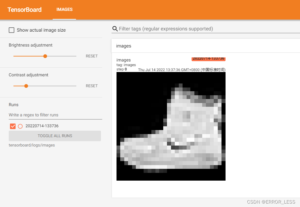
  tf.summary.image("images", img, step=0)

到此为止，运行之后便可以查看单个图像了：可以调节亮度和对比度
在这里插入图片描述

2.3 加上可视化25张图片代码样例

#!/usr/bin/env python
# -*- coding: utf-8 -*-
# @Time : 2022/7/14 12:40
# @Author : hqc
# @File : image_usage.py
# @Software: PyCharm

### import necessary modules

from datetime import datetime
import io # related to file reading and writing
import itertools # used to operate the iterator
#from packaging import version # 语义化版本
#from six.moves import range # six is used to compatible with py2 and py3

import tensorflow as tf
from tensorflow import keras

import matplotlib.pyplot as plt
import numpy as np
import sklearn.metrics # 评价指标

print("TensorFlow version: ", tf.__version__)

### download Fashion-MNIST dataset
# Download the data. The data is already divided into train and test.
# The labels are integers representing classes.
fashion_mnist = keras.datasets.fashion_mnist
(train_images, train_labels), (test_images, test_labels) = \
    fashion_mnist.load_data()

# Names of the integer classes, i.e., 0 -> T-short/top, 1 -> Trouser, etc.
class_names = ['T-shirt/top', 'Trouser', 'Pullover', 'Dress', 'Coat',
    'Sandal', 'Shirt', 'Sneaker', 'Bag', 'Ankle boot']

### make sure the shape of train data
print("Shape: ", train_images[0].shape)
print("Label: ", train_labels[0], "->", class_names[train_labels[0]])
# Shape:  (28, 28)
# Label:  9 -> Ankle boot

'''
tf.summary.image() API needs to contain 4-tensors:(batch_size, height, width, channels)
so we should reshape train data, because we just log one image so batch_size set to -1;
and the image is gray-scaled, so channels set to 1.
'''
# Reshape a image for the Summary API.
img = np.reshape(train_images[0], (-1, 28, 28, 1))
# Reshape 25 images for the Summary API.
images = np.reshape(train_images[0:25], (-1, 28, 28, 1))

### set the log directory
logdir = "logs/images/" + datetime.now().strftime("%Y%m%d-%H%M%S")
# Creates a file writer for the log directory.
file_writer = tf.summary.create_file_writer(logdir)

# Using the file writer, log the reshaped image.
with file_writer.as_default():
  tf.summary.image("image", img, step=0)
  tf.summary.image("25 training data examples", images, max_outputs=25, step=0)

在这里插入图片描述

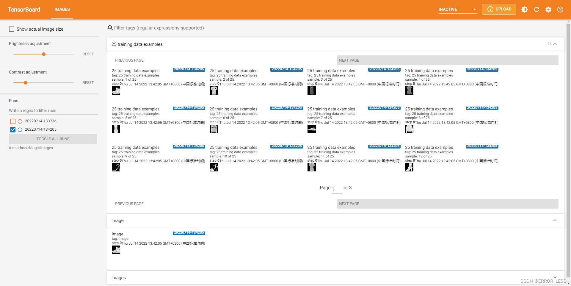
可见，可视化成功！

2.4 记录`matplotlib`生成的图像

需要一些样板代码来将图转换为张量，随后便可继续处理。
完整代码如下：

#!/usr/bin/env python
# -*- coding: utf-8 -*-
# @Time : 2022/7/14 13:49
# @Author : hqc
# @File : plot_to_image_usage.py
# @Software: PyCharm

### import necessary modules

from datetime import datetime
import io # related to file reading and writing
import itertools # used to operate the iterator
#from packaging import version # 语义化版本
#from six.moves import range # six is used to compatible with py2 and py3

import tensorflow as tf
from tensorflow import keras

import matplotlib.pyplot as plt
import numpy as np
import sklearn.metrics # 评价指标

print("TensorFlow version: ", tf.__version__)

### download Fashion-MNIST dataset
# Download the data. The data is already divided into train and test.
# The labels are integers representing classes.
fashion_mnist = keras.datasets.fashion_mnist
(train_images, train_labels), (test_images, test_labels) = \
    fashion_mnist.load_data()

# Names of the integer classes, i.e., 0 -> T-short/top, 1 -> Trouser, etc.
class_names = ['T-shirt/top', 'Trouser', 'Pullover', 'Dress', 'Coat',
    'Sandal', 'Shirt', 'Sneaker', 'Bag', 'Ankle boot']

### set the log directory
logdir = "logs/plots/" + datetime.now().strftime("%Y%m%d-%H%M%S")
# Creates a file writer for the log directory.
file_writer = tf.summary.create_file_writer(logdir)

### convert plot to image
def plot_to_image(figure):
  """Converts the matplotlib plot specified by 'figure' to a PNG image and
  returns it. The supplied figure is closed and inaccessible after this call."""
  # Save the plot to a PNG in memory.
  buf = io.BytesIO()
  plt.savefig(buf, format='png')
  #plt.close(figure)# Closing the figure prevents it from being displayed directly inside the notebook.
  buf.seek(0) # read from the top of this file
  # Convert PNG buffer to TF image
  image = tf.image.decode_png(buf.getvalue(), channels=4)
  # Add the batch dimension
  image = tf.expand_dims(image, 0)
  return image

def image_grid():
  """Return a 5x5 grid of the MNIST images as a matplotlib figure."""
  # Create a figure to contain the plot.
  figure = plt.figure(figsize=(10,10))
  for i in range(25):
    # Start next subplot.
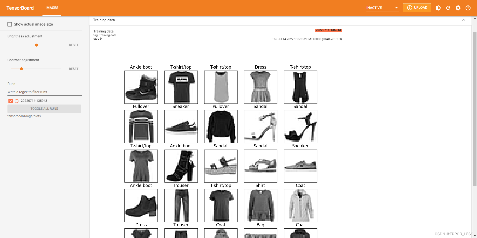
    plt.subplot(5, 5, i + 1, title=class_names[train_labels[i]])
    plt.xticks([])
    plt.yticks([])
    plt.grid(False)
    plt.imshow(train_images[i], cmap=plt.cm.binary)

  return figure

# Prepare the plot
figure = image_grid()
# Convert to image and log
with file_writer.as_default():
  tf.summary.image("Training data", plot_to_image(figure), step=0)

运行结果查看：
在这里插入图片描述

2.5 高阶应用：模型训练中构建图像分类器

这种方式看不大懂，仅附上能够运行的完整代码及运行结果

完整代码：

#!/usr/bin/env python
# -*- coding: utf-8 -*-
# @Time : 2022/7/14 14:50
# @Author : hqc
# @File : model_with_image_usage.py
# @Software: PyCharm

### import necessary modules

from datetime import datetime
import io # related to file reading and writing
import itertools # used to operate the iterator
#from packaging import version # 语义化版本
from six.moves import range # six is used to compatible with py2 and py3

import tensorflow as tf
from tensorflow import keras

import matplotlib.pyplot as plt
import numpy as np
import sklearn.metrics # 评价指标

print("TensorFlow version: ", tf.__version__)

### download Fashion-MNIST dataset
# Download the data. The data is already divided into train and test.
# The labels are integers representing classes.
fashion_mnist = keras.datasets.fashion_mnist
(train_images, train_labels), (test_images, test_labels) = \
    fashion_mnist.load_data()

# Names of the integer classes, i.e., 0 -> T-short/top, 1 -> Trouser, etc.
class_names = ['T-shirt/top', 'Trouser', 'Pullover', 'Dress', 'Coat',
    'Sandal', 'Shirt', 'Sneaker', 'Bag', 'Ankle boot']

### define and compile a model
model = keras.models.Sequential([
    keras.layers.Flatten(input_shape=(28, 28)),
    keras.layers.Dense(32, activation='relu'),
    keras.layers.Dense(10, activation='softmax')
])

model.compile(
    optimizer='adam',
    loss='sparse_categorical_crossentropy',
    metrics=['accuracy']
)


def plot_confusion_matrix(cm, class_names):
  """
  Returns a matplotlib figure containing the plotted confusion matrix.

  Args:
    cm (array, shape = [n, n]): a confusion matrix of integer classes
    class_names (array, shape = [n]): String names of the integer classes
  """
  figure = plt.figure(figsize=(8, 8))
  plt.imshow(cm, interpolation='nearest', cmap=plt.cm.Blues)
  plt.title("Confusion matrix")
  plt.colorbar()
  tick_marks = np.arange(len(class_names))
  plt.xticks(tick_marks, class_names, rotation=45)
  plt.yticks(tick_marks, class_names)

  # Normalize the confusion matrix.
  cm = np.around(cm.astype('float') / cm.sum(axis=1)[:, np.newaxis], decimals=2)

  # Use white text if squares are dark; otherwise black.
  threshold = cm.max() / 2.
  for i, j in itertools.product(range(cm.shape[0]), range(cm.shape[1])):
    color = "white" if cm[i, j] > threshold else "black"
    plt.text(j, i, cm[i, j], horizontalalignment="center", color=color)

  plt.tight_layout()
  plt.ylabel('True label')
  plt.xlabel('Predicted label')
  return figure

### set the log directory
logdir = "logs/model/" + datetime.now().strftime("%Y%m%d-%H%M%S")
# Define the basic TensorBoard callback.
tensorboard_callback = keras.callbacks.TensorBoard(log_dir=logdir)
file_writer_cm = tf.summary.create_file_writer(logdir + '/cm')

### convert plot to image
def plot_to_image(figure):
  """Converts the matplotlib plot specified by 'figure' to a PNG image and
  returns it. The supplied figure is closed and inaccessible after this call."""
  # Save the plot to a PNG in memory.
  buf = io.BytesIO()
  plt.savefig(buf, format='png')
  #plt.close(figure)# Closing the figure prevents it from being displayed directly inside the notebook.
  buf.seek(0) # read from the top of this file
  # Convert PNG buffer to TF image
  image = tf.image.decode_png(buf.getvalue(), channels=4)
  # Add the batch dimension
  image = tf.expand_dims(image, 0)
  return image

def log_confusion_matrix(epoch, logs):
  # Use the model to predict the values from the validation dataset.
  test_pred_raw = model.predict(test_images)
  test_pred = np.argmax(test_pred_raw, axis=1)

  # Calculate the confusion matrix.
  cm = sklearn.metrics.confusion_matrix(test_labels, test_pred)
  # Log the confusion matrix as an image summary.
  figure = plot_confusion_matrix(cm, class_names=class_names)
  cm_image = plot_to_image(figure)

  # Log the confusion matrix as an image summary.
  with file_writer_cm.as_default():
    tf.summary.image("Confusion Matrix", cm_image, step=epoch)

# Define the per-epoch callback.
cm_callback = keras.callbacks.LambdaCallback(on_epoch_end=log_confusion_matrix)

# Train the classifier.
model.fit(
    train_images,
    train_labels,
    epochs=5,
    verbose=0, # Suppress chatty output
    callbacks=[tensorboard_callback, cm_callback],
    validation_data=(test_images, test_labels),
)

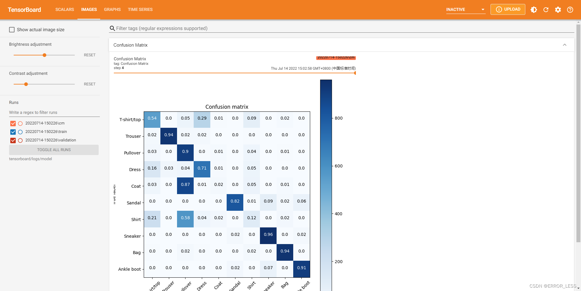
运行结果：
在这里插入图片描述

3 Graph：查看模型图

3.1 概述

官方文档

TensorBoard 的 GRAPH仪表盘是检查 TensorFlow 模型的强大工具。您可以快速查看模型结构的预览图，并确保其符合您的预期想法。您还可以查看操作级图以了解 TensorFlow 如何理解您的程序。检查操作级图可以使您深入了解如何更改模型。例如，如果训练进度比预期的慢，则可以重新设计模型。

本教程简要概述了如何在 TensorBoard 的 GRAPH仪表板中生成图诊断数据并将其可视化。您将为 Fashion-MNIST 数据集定义和训练一个简单的 Keras 序列模型，并学习如何记录和检查模型图。您还将使用跟踪API为使用新的 tf.function 注释创建的函数生成图数据。

本节以minst训练为例，见tensorboard可视化工具使用示例（tf2.6）。

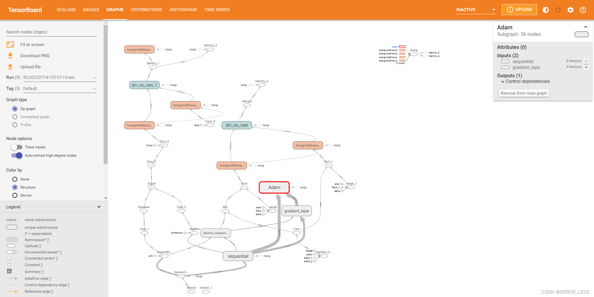
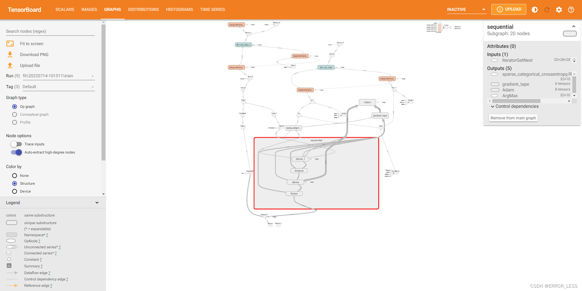
3.2 执行图：`op-level graph`

默认情况下，TensorBoard 显示 op-level图。（在左侧，您可以看到已选择 “Default” 标签。）请注意，图是倒置的。数据从下到上流动，因此与代码相比是上下颠倒的。但是，您可以看到该图与 Keras 模型定义紧密匹配，并具有其他计算节点的额外边缘。

图通常很大，因此您可以操纵图的可视化效果：

滚动来放大和缩小
拖动进行图的平移
双击进行节点扩展（一个节点可以是其他节点的容器）

您还可以通过单击节点来查看元数据。这使您可以查看输入，输出，形状和其他详细信息。
在这里插入图片描述

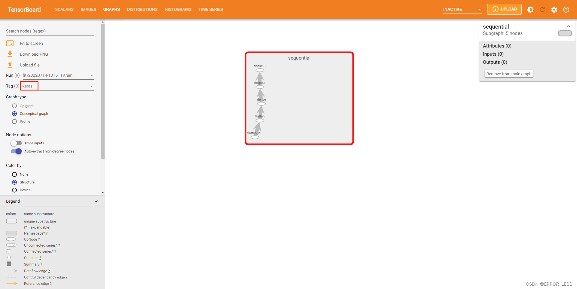
3.3 概念图

除了执行图，TensorBoard 还显示一个“概念图”。这只是 Keras 模型的视图。如果您要重新使用保存的模型并且想要检查或验证其结构，这可能会很有用。

要查看概念图，请选择 “keras” 标签。在此示例中，您将看到一个折叠的 Sequential 节点。双击节点以查看模型的结构：
在这里插入图片描述

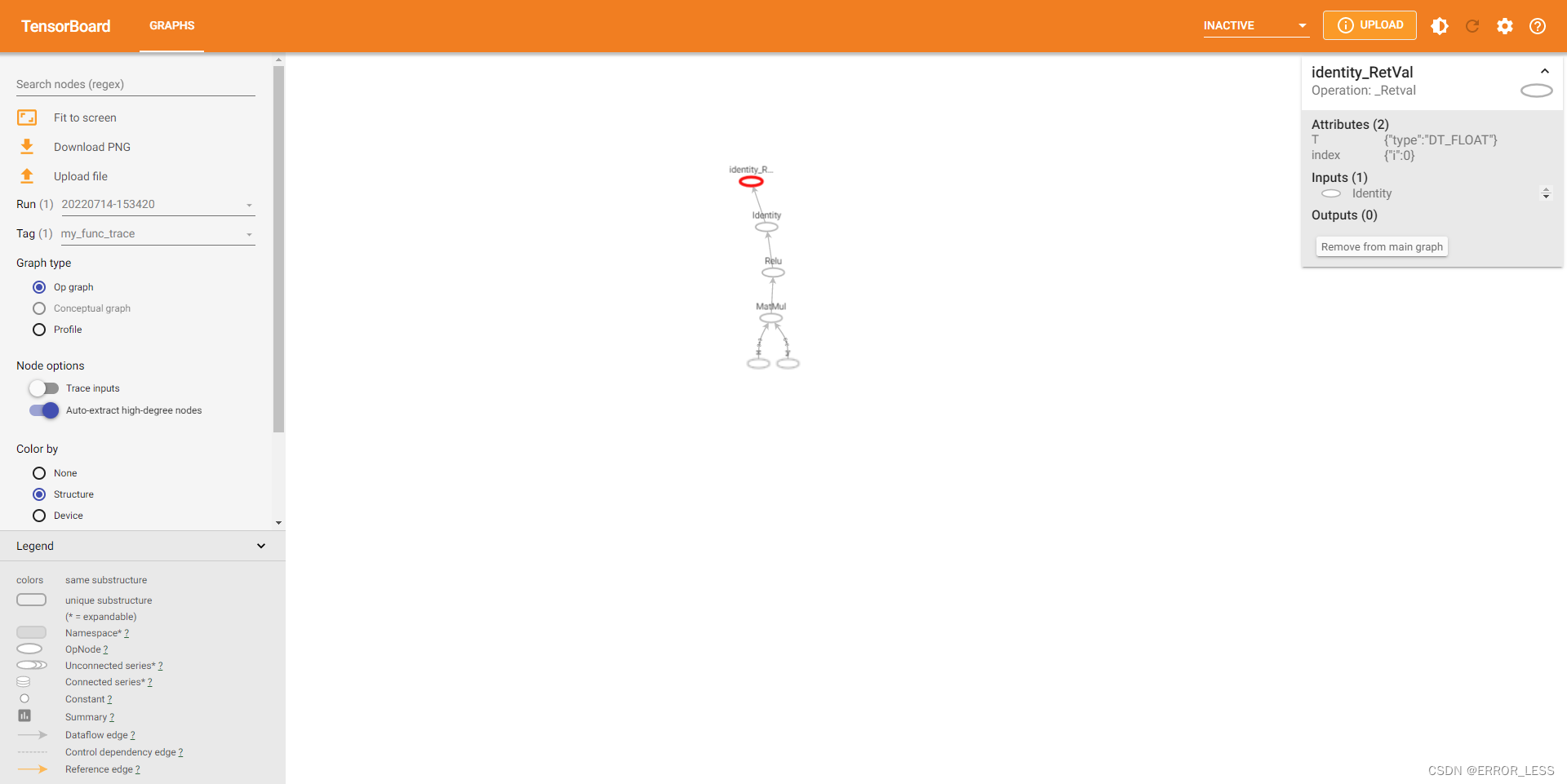
3.4 高阶应用：`tf.function`的图

到目前为止的示例已经描述了 Keras 模型的图，其中这些图是通过定义 Keras 层并调用 Model.fit() 创建的。

您可能会遇到需要使用 tf.function 注释来[autograph]的情况，即将 Python 计算函数转换为高性能 TensorFlow 图。对于这些情况，您可以使用 TensorBoard 中的 TensorFlow Summary Trace API 记录签名函数以进行可视化。

要使用 Summary Trace API ，请执行以下操作:

使用 tf.function 定义和注释功能
在函数调用站点之前立即使用 tf.summary.trace_on()
通过传递 profiler=True 将配置文件信息（内存，CPU时间）添加到图中
使用摘要文件编写器，调用 tf.summary.trace_export() 保存日志数据

然后，您可以使用 TensorBoard 查看函数的行为。

完整代码如下：

#!/usr/bin/env python
# -*- coding: utf-8 -*-
# @Time : 2022/7/13 20:48
# @Author : hqc
# @File : tensorboard_usage.py
# @Software: PyCharm

# import necessary modules
import tensorflow as tf
from datetime import datetime

# The function to be traced.
@tf.function
def my_func(x, y):
  # A simple hand-rolled layer.
  return tf.nn.relu(tf.matmul(x, y))

# Set up logging.
stamp = datetime.now().strftime("%Y%m%d-%H%M%S")
logdir = 'logs/func/%s' % stamp
writer = tf.summary.create_file_writer(logdir)

# Sample data for your function.
x = tf.random.uniform((3, 3))
y = tf.random.uniform((3, 3))

# Bracket the function call with
# tf.summary.trace_on() and tf.summary.trace_export().
tf.summary.trace_on(graph=True, profiler=True)
# Call only one tf.function when tracing.
z = my_func(x, y)
with writer.as_default():
  tf.summary.trace_export(
      name="my_func_trace",
      step=0,
      profiler_outdir=logdir)

查看运行结果：
在这里插入图片描述

4 Text：查看文本信息

4.1 概述

官方文档

可以很简单地在tensorboard中查看任意文本。

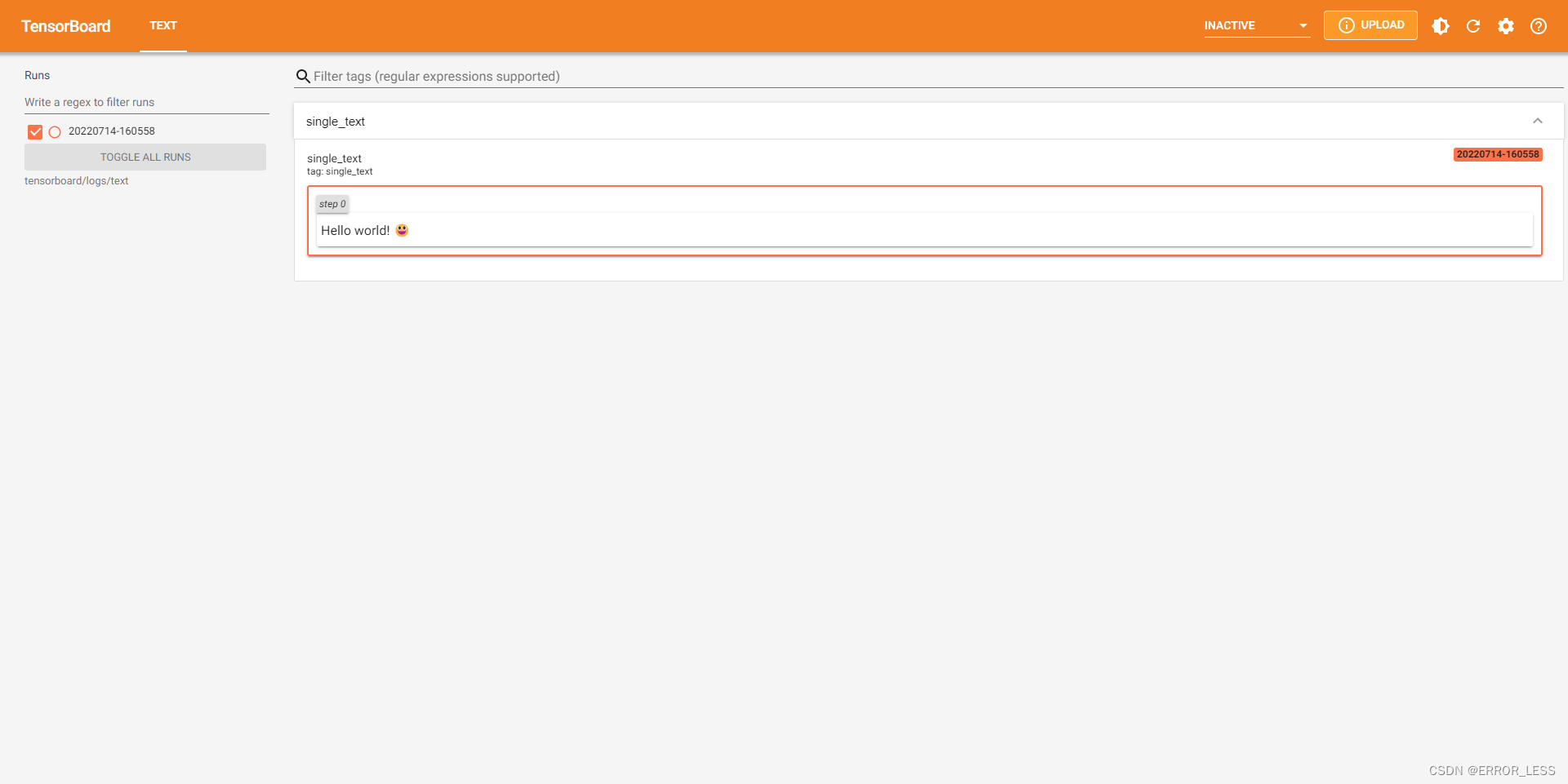
4.2 记录单条文本

完整代码如下：

#!/usr/bin/env python
# -*- coding: utf-8 -*-
# @Time : 2022/7/14 16:03
# @Author : hqc
# @File : text_single_usage.py
# @Software: PyCharm

### import necessary modules

import tensorflow as tf
from datetime import datetime


print("TensorFlow version: ", tf.__version__)

### define your text
my_text = "Hello world! 😃"

### Sets up a timestamped log directory.
logdir = "logs/text/" + datetime.now().strftime("%Y%m%d-%H%M%S")
# Creates a file writer for the log directory.
file_writer = tf.summary.create_file_writer(logdir)

# Using the file writer, log the text.
with file_writer.as_default():
  tf.summary.text("single_text", my_text, step=0)

运行结果查看：
在这里插入图片描述

4.3 记录多条文本数据流

在命令行中启动tensorboard可以通过--samples_per_plugin来控制采样频率。

完整代码如下：

#!/usr/bin/env python
# -*- coding: utf-8 -*-
# @Time : 2022/7/14 16:11
# @Author : hqc
# @File : text_multi_usage.py
# @Software: PyCharm

### import necessary modules

import tensorflow as tf
from datetime import datetime


print("TensorFlow version: ", tf.__version__)

### Sets up a timestamped log directory.
logdir = "logs/texts/" + datetime.now().strftime("%Y%m%d-%H%M%S")
# Creates a file writer for the log directory.
file_writer = tf.summary.create_file_writer(logdir)

# Using the file writer, log the text.
with file_writer.as_default():
    with tf.name_scope("name_scope_1"):
        for step in range(20):
            tf.summary.text("a_stream_of_text", f"Hello from step {step}", step=step)
            tf.summary.text("another_stream_of_text", f"This can be kept separate {step}", step=step)
    with tf.name_scope("name_scope_2"):
        tf.summary.text("just_from_step_0", "This is an important announcement from step 0", step=0)

运行结果查看：tensorboard --logdir tensorboard/logs/texts --samples_per_plugin 'text=5'；
参数text=5表示20轮循环中采样其中5个。
在这里插入图片描述

4.4 高阶应用：Markdown

完整代码：

#!/usr/bin/env python
# -*- coding: utf-8 -*-
# @Time : 2022/7/14 16:19
# @Author : hqc
# @File : text_markdown_usage.py
# @Software: PyCharm


### import necessary modules

import tensorflow as tf
from datetime import datetime
import json

print("TensorFlow version: ", tf.__version__)

### Sets up a timestamped log directory.
logdir = "logs/markdown/" + datetime.now().strftime("%Y%m%d-%H%M%S")
# Creates a file writer for the log directory.
file_writer = tf.summary.create_file_writer(logdir)

some_obj_worth_noting = {
  "tfds_training_data": {
      "name": "mnist",
      "split": "train",
      "shuffle_files": "True",
  },
  "keras_optimizer": {
      "name": "Adagrad",
      "learning_rate": "0.001",
      "epsilon": 1e-07,
  },
  "hardware": "Cloud TPU",
}

# TODO: Update this example when TensorBoard is released with
# https://github.com/tensorflow/tensorboard/pull/4585
# which supports fenced codeblocks in Markdown.
def pretty_json(hp):
  json_hp = json.dumps(hp, indent=2)
  return "".join("\t" + line for line in json_hp.splitlines(True))
# 不知道这个函数是在干嘛。

markdown_text = """
### Markdown Text

TensorBoard supports basic markdown syntax, including:

    preformatted code

**bold text**

| and | tables |
| ---- | ---------- |
| among | others |
"""

with file_writer.as_default():
  tf.summary.text("run_params", pretty_json(some_obj_worth_noting), step=0)
  tf.summary.text("markdown_jubiliee", markdown_text, step=0)

运行结果查看：
在这里插入图片描述
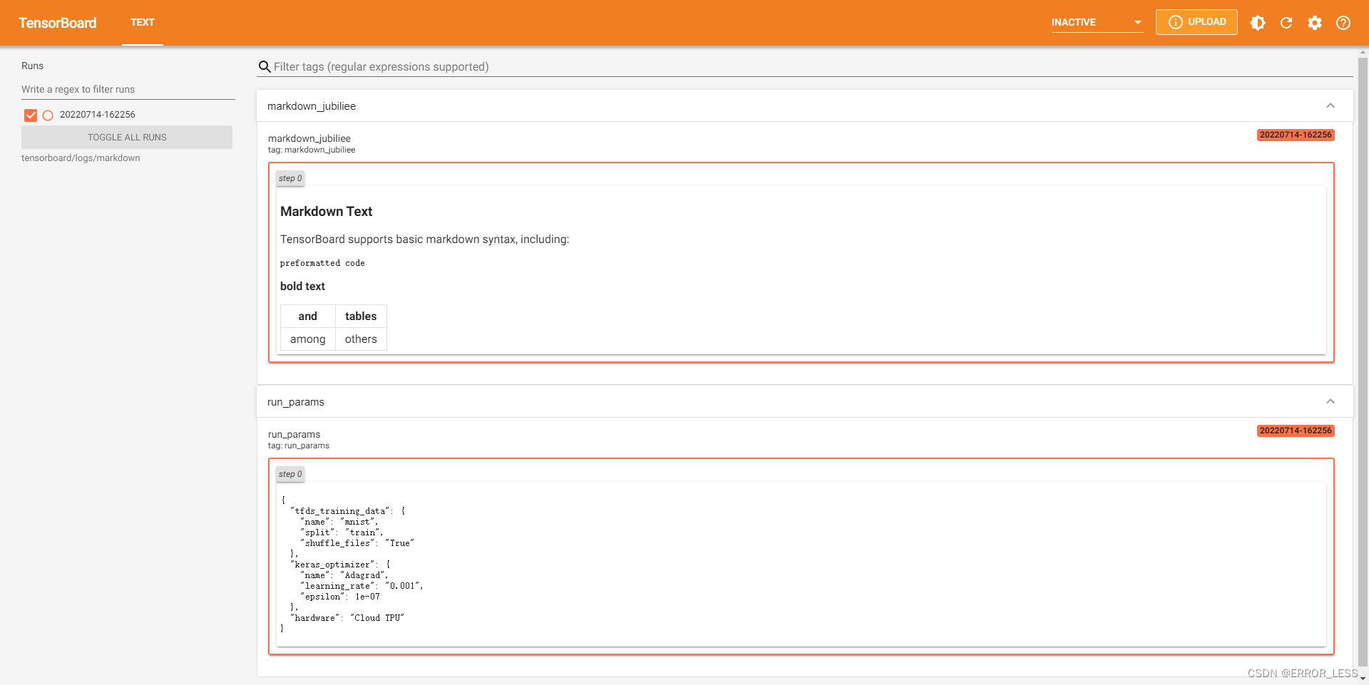
可见markdown文本可以在tensorboard中展现。

5 Profiler：剖析模型的性能

5.1 概述

官方文档
这里想插播一下：尽量还是看英文文档吧~中文文档和英文文档相差太多了！

在机器学习中性能十分重要。TensorFlow 有一个内置的性能分析器可以使您不用费力记录每个操作的运行时间。然后您就可以在 TensorBoard 的 Profile Plugin 中对配置结果进行可视化。本教程侧重于 GPU ，但性能分析插件也可以按照云 TPU 工具来在 TPU 上使用。

本教程提供了非常基础的示例以帮助您学习如何在开发 Keras 模型时启用性能分析器。您将学习如何使用 Keras TensorBoard 回调函数来可视化性能分析结果。“其他性能分析方式”中提到的 Profiler API 和 Profiler Server 允许您分析非 Keras TensorFlow 的任务。

5.2 代码示例

可能得先安装一下（不知道是否自带）：pip install -U tensorboard_plugin_profile

#!/usr/bin/env python
# -*- coding: utf-8 -*-
# @Time : 2022/7/14 16:39
# @Author : hqc
# @File : profiler_usage.py
# @Software: PyCharm

### import necessary modules

from datetime import datetime
from packaging import version

import os

import tensorflow as tf

print("TensorFlow version: ", tf.__version__)

import tensorflow_datasets as tfds
tfds.disable_progress_bar()

# device_name = tf.test.gpu_device_name()
# if not device_name:
#   raise SystemError('GPU device not found')
# print('Found GPU at: {}'.format(device_name))

### load the mnist dataset and split it into training and testing sets
(ds_train, ds_test), ds_info = tfds.load(
    'mnist',
    split=['train', 'test'],
    shuffle_files=True,
    as_supervised=True,
    with_info=True,
)

### Preprocess the training and test data by normalizing pixel values to be between 0 and 1.
def normalize_img(image, label):
  """Normalizes images: `uint8` -> `float32`."""
  return tf.cast(image, tf.float32) / 255., label

ds_train = ds_train.map(normalize_img)
ds_train = ds_train.batch(128)

ds_test = ds_test.map(normalize_img)
ds_test = ds_test.batch(128)

### Create the image classification model using Keras.
model = tf.keras.models.Sequential([
  tf.keras.layers.Flatten(input_shape=(28, 28, 1)),
  tf.keras.layers.Dense(128,activation='relu'),
  tf.keras.layers.Dense(10, activation='softmax')
])
model.compile(
    loss='sparse_categorical_crossentropy',
    optimizer=tf.keras.optimizers.Adam(0.001),
    metrics=['accuracy']
)

### Sets up a timestamped log directory.
logdir = "logs/profiler/" + datetime.now().strftime("%Y%m%d-%H%M%S")
### Create a TensorBoard callback
profiler_callback = tf.keras.callbacks.TensorBoard(log_dir = logdir,
                                                 histogram_freq = 1,
                                                 profile_batch = '500,520')
### training
model.fit(ds_train,
          epochs=2,
          validation_data=ds_test,
          callbacks = [profiler_callback])

代码说明：由于使用测试的电脑没有GPU，因此将检测GPU那部分注释掉。

4.3 运行结果

在这里插入图片描述
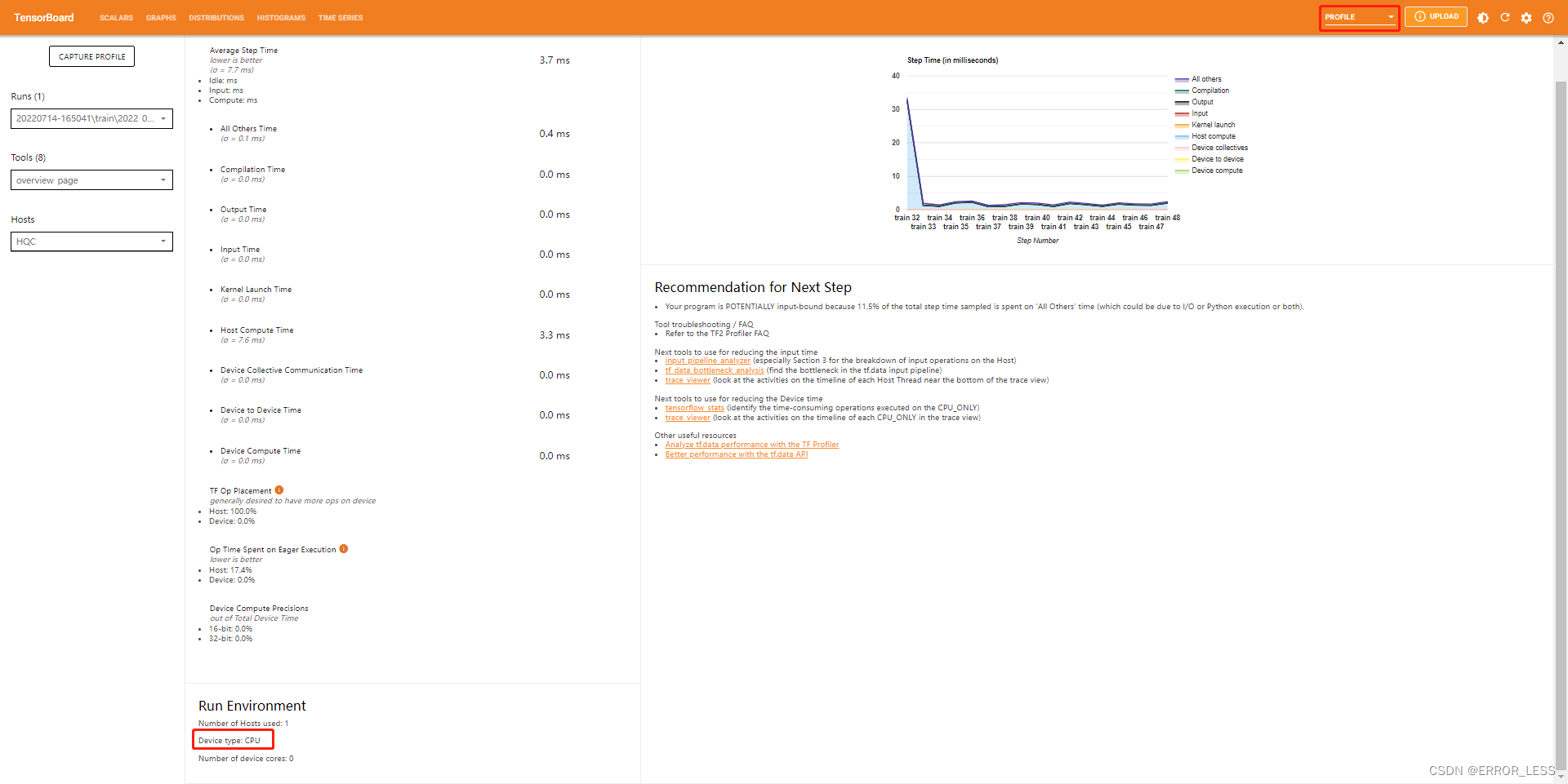
操作和官方文档不一致（可能是版本原因）的是，标题栏那里没有PROFILE选项，在右上角的下拉菜单里边有。

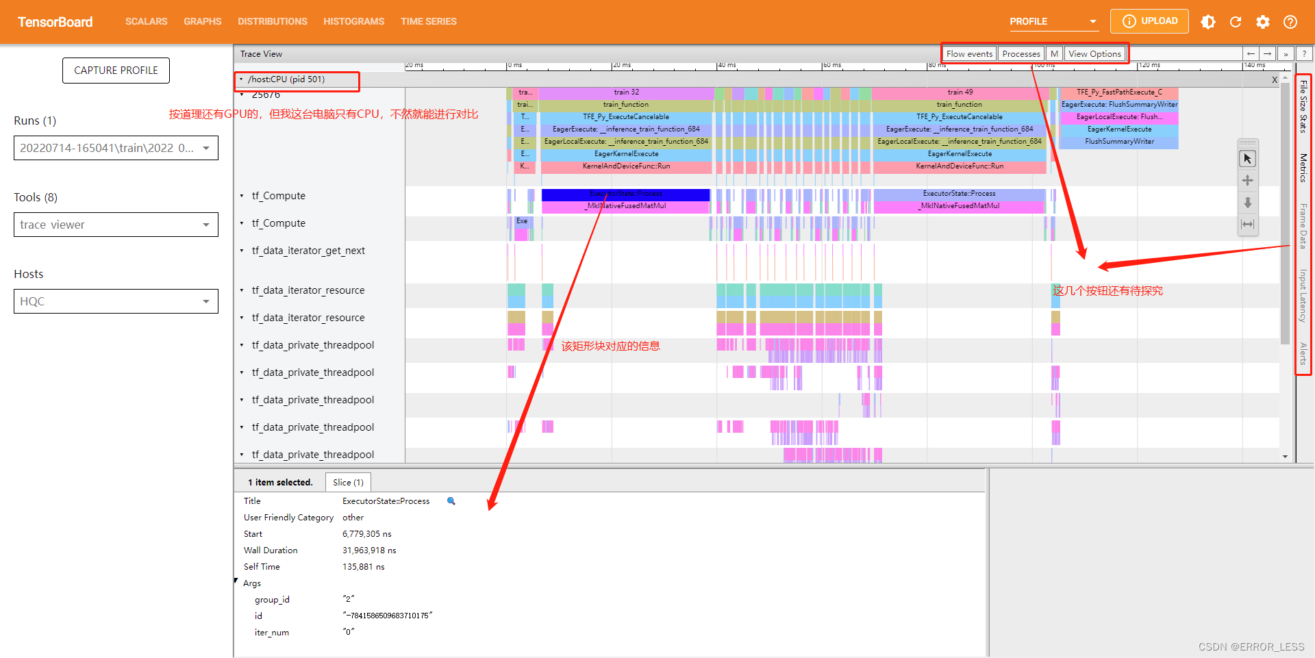
界面第一眼最下面可以看到，模型使用的是CPU进行训练，所有评估指标也都是CPU上的。

4.4 界面详细指标说明

4.4.0 概述

overview_page界面可以看到每一个部分所花的时间、随训练的时间变化、运行环境、改进建议等

Trace Viewer可以查看输入流水线中CPU和GPU上发生了什么障碍。

4.4.1 总界面（`overview_page`）

左侧包括Profiler设置（CAPTURE PROFILE），8种工具选项（可以查看8种不同的界面），以及运行的主机名（Hosts）。
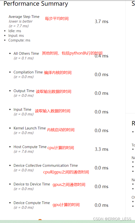
中间一列有性能总览，包括每步平均时间以及编译时间、输入时间、输出时间、主机计算时间、设备计算时间、设备与设备之间的通信时间等等。
右侧有一个随着训练步数各种时间的变化折线图。
右下角会给出你下一步训练的推荐建议去优化模型。比如，这次实验给出的建议是：其他时间花费的太多，占了11.5%，可能的原因是读取和python执行的问题。
下方会给出当前训练的运行环境。

4.4.2 `trace_viewer`

可以查看输入流水线中CPU和GPU上执行的情况，是否发生了什么障碍
在这里插入图片描述

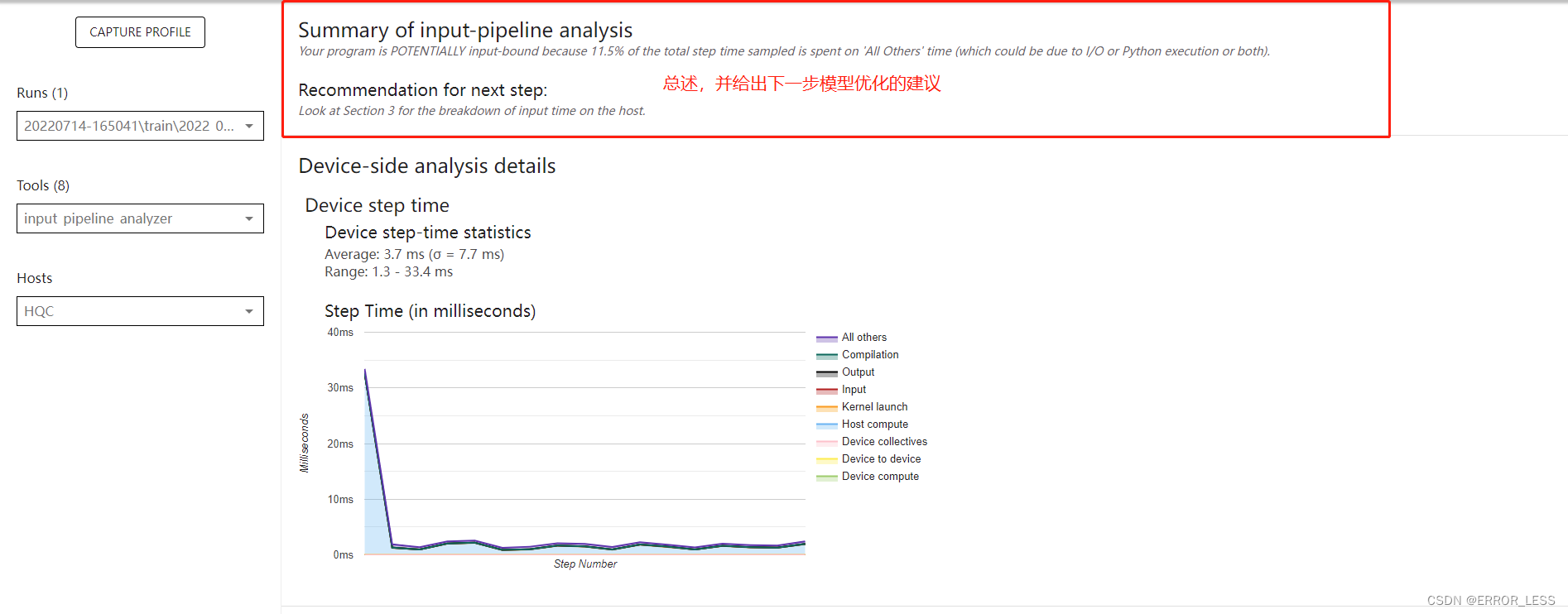
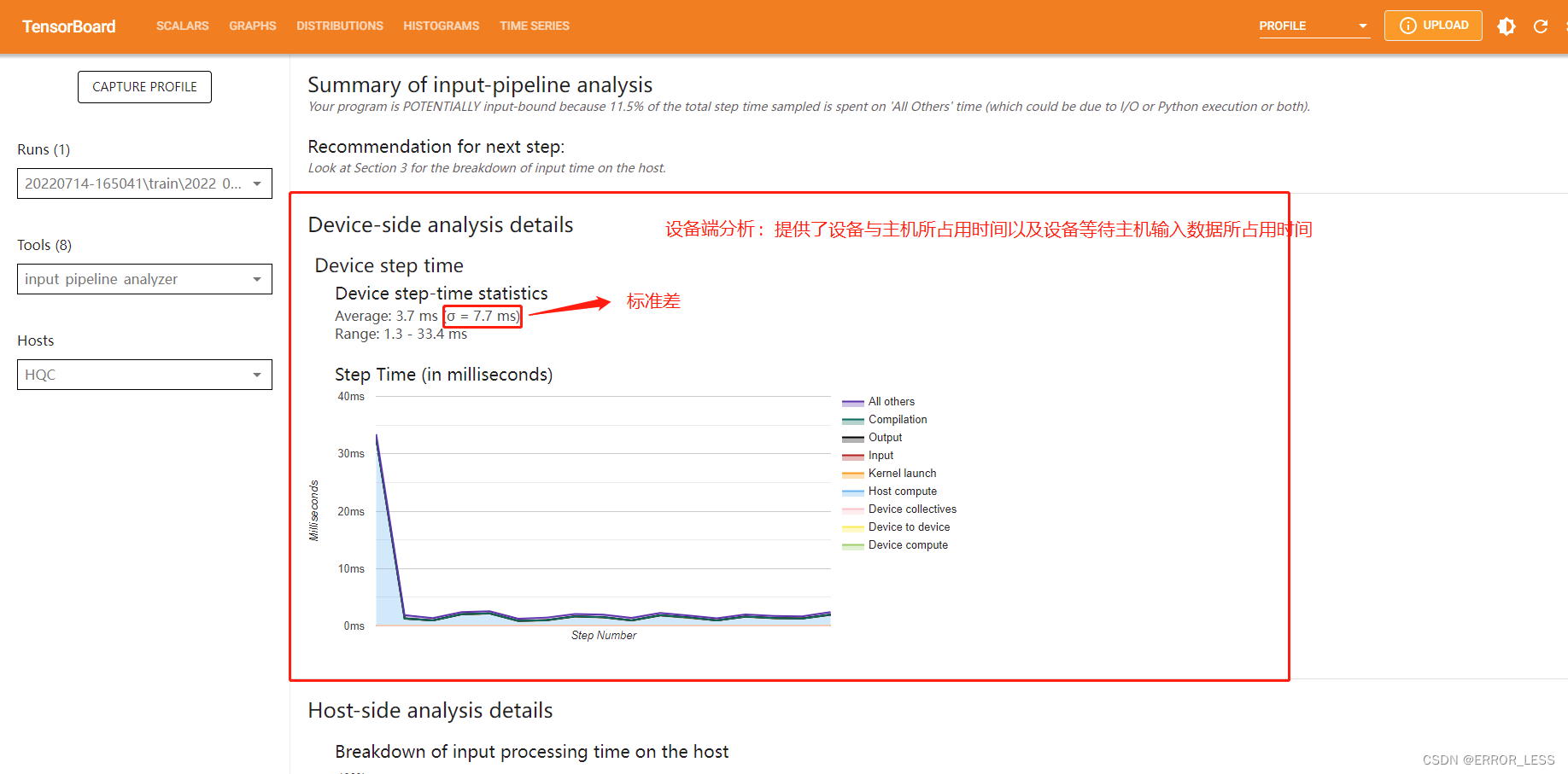
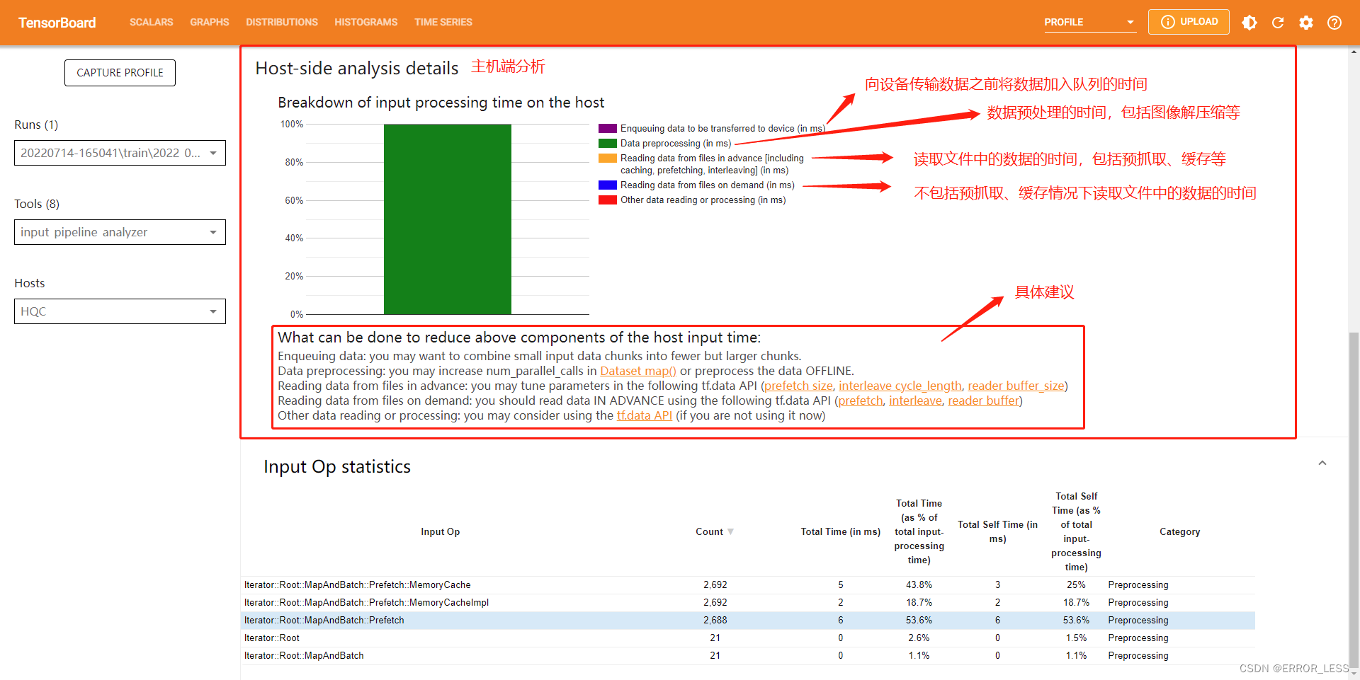
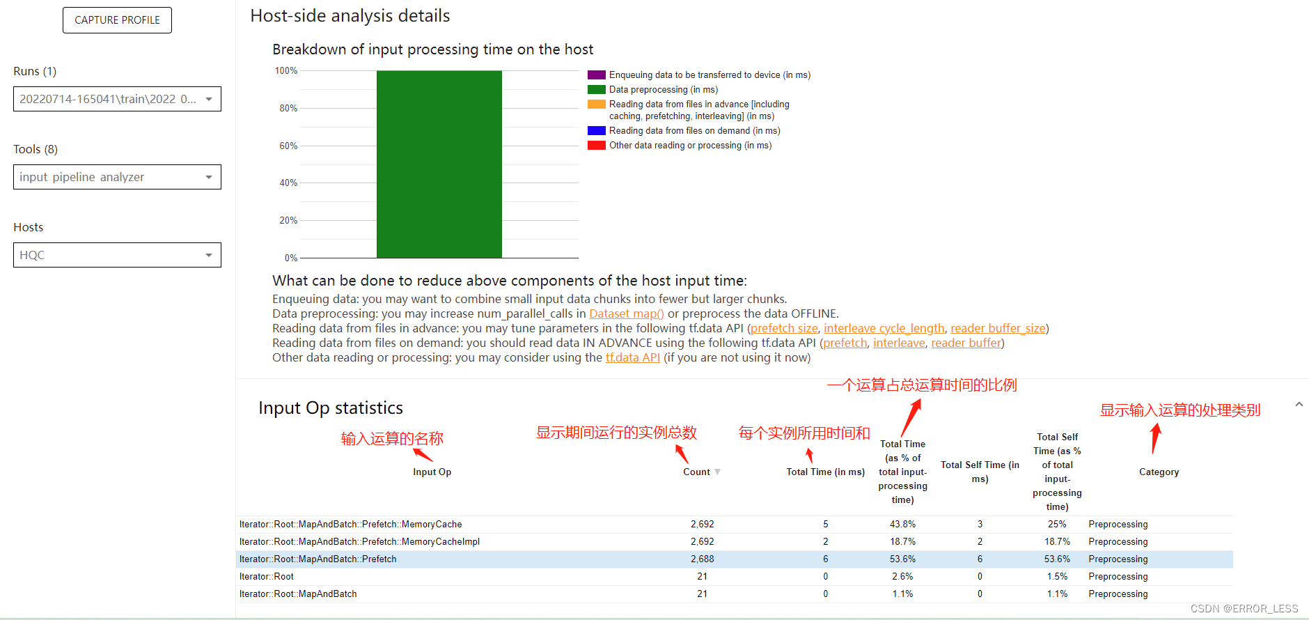
4.4.3 `Input pipeline analyzer`

输入流水线分析器。

我们将输入数据经过处理之后的输出作为下一个数据处理模块的输入最后得到最终输出的数据处理方式称为输入流水线。

对于低效的输入流水线，有几个关键考虑点：

数据读取
数据处理
数据在cpu和gpu之间传输

在这里插入图片描述

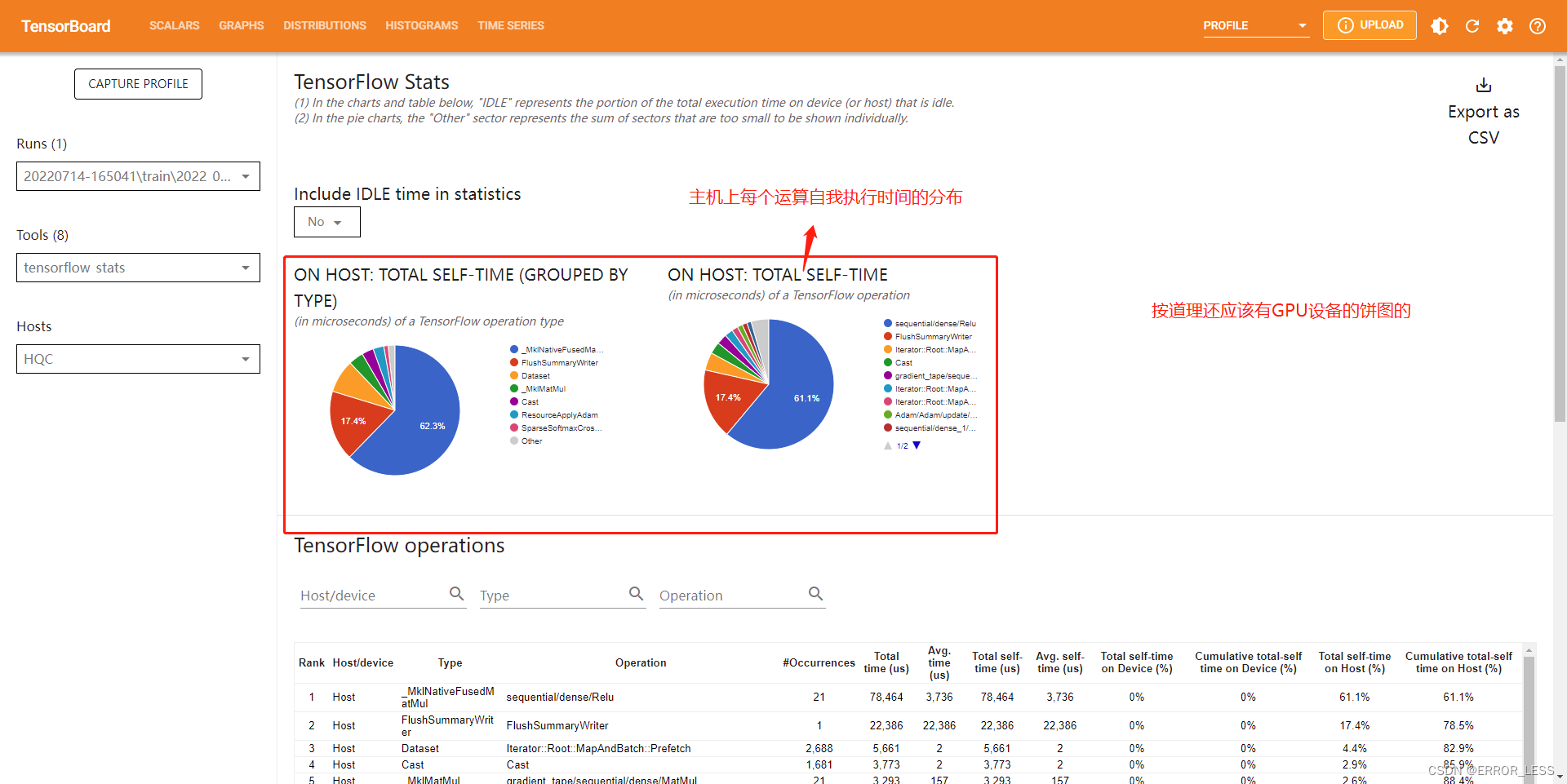
4.4.4 `TensorFlow Stats`

在这里插入图片描述

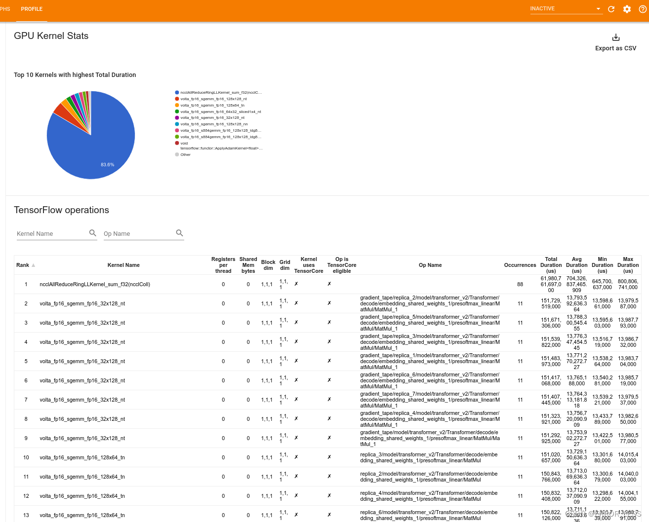
4.4.5 `GPU Kernel Stats`

此工具可以显示性能统计信息以及每个 GPU 加速内核的源运算。（什么意思，不懂啊）
在这里插入图片描述

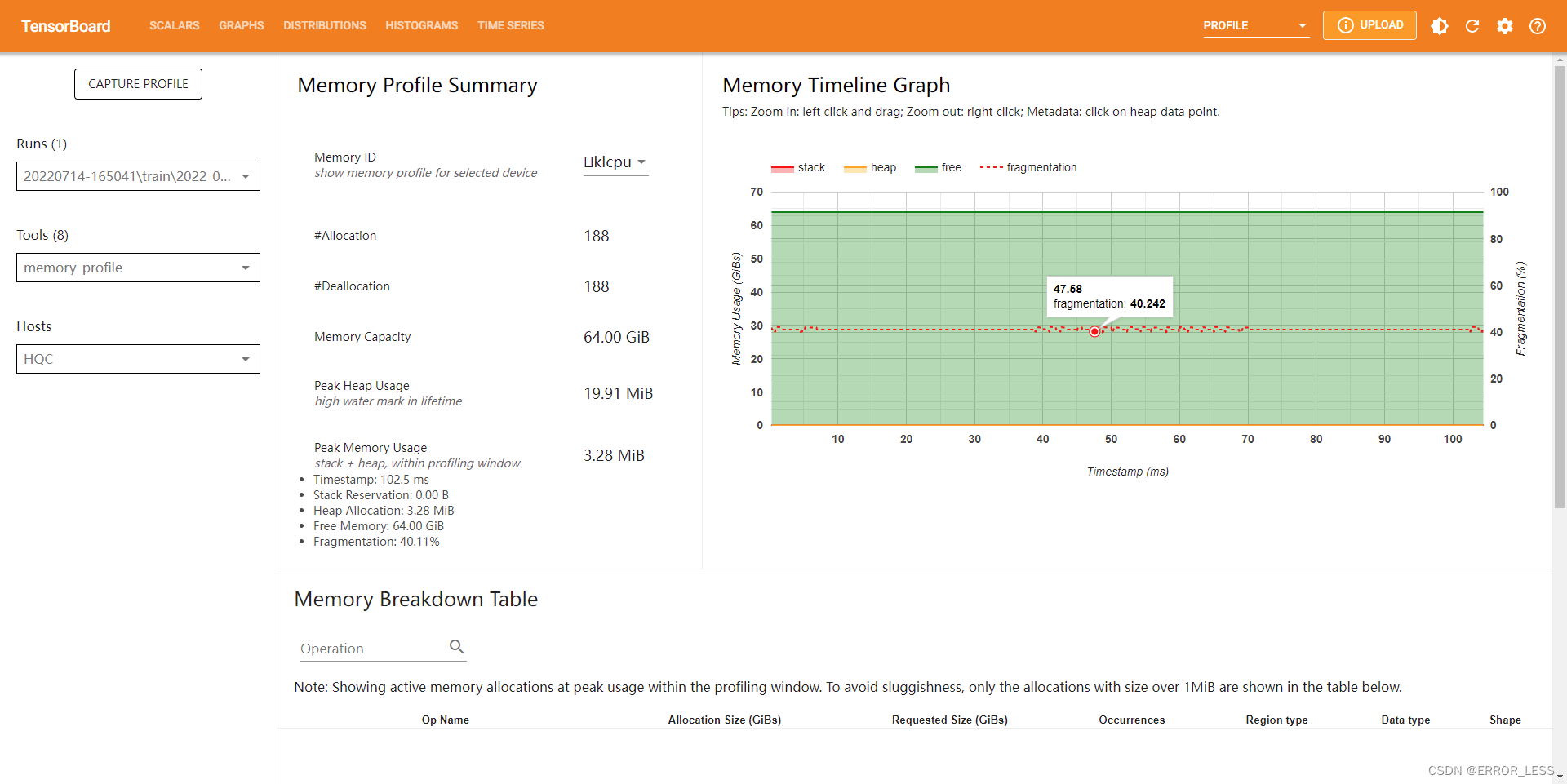
4.4.6 `Memory Profile`

显示了内存使用量（以 GiB 为单位）
在这里插入图片描述

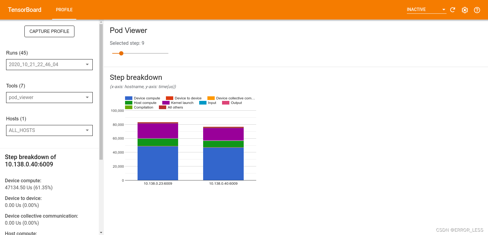
4.4.7 `Pod viewer`

显示了所有工作进程中训练步骤的详细情况。
在这里插入图片描述

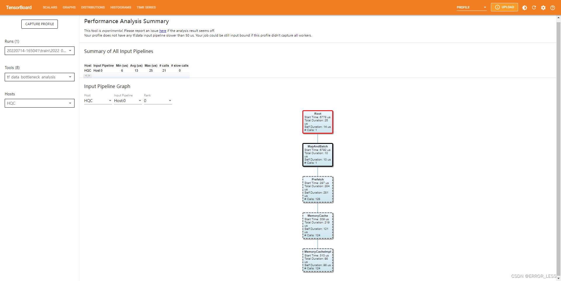
4.4.8 `tf.data bottleneck analysis`

实验性的组件
在这里插入图片描述

4.5 总结

比较有用的可能就是overview_page了，后面那些太偏细节了，高阶用户可以考虑。

ERROR_LESS

关注

4
点赞
踩
28

收藏

觉得还不错? 一键收藏
0
评论
tensorboard使用界面介绍以及使用方法（看这篇就够了，都有源码可以直接测试）

参考文档机器学习总是涉及理解关键指标，例如损失(loss)，以及它们如何随着训练的进行而变化。例如，这些指标可以帮助您了解模型是否过拟合，或者是否不必要地训练了太长时间。您可能需要比较不同训练中的这些指标，以帮助调试和改善模型。重新训练回归模型并记录自定义学习率。使用创建文件编写器。定义自定义学习率函数。这将传递给Keras回调。在学习率函数内部，使用记录自定义学习率。将回调传递给Model.fit()。#!"""运行后发现log里边多了一个metrics参考文档使用可视化层权重。...
复制链接

扫一扫