


Python Basics with Numpy (optional assignment)
Welcome to your first assignment. This exercise gives you a brief introduction to Python. Even if you’ve used Python before, this will help familiarize you with functions we’ll need.
Instructions:
- You will be using Python 3.
- Avoid using for-loops and while-loops, unless you are explicitly told to do so.
- Do not modify the (# GRADED FUNCTION [function name]) comment in some cells. Your work would not be graded if you change this. Each cell containing that comment should only contain one function.
- After coding your function, run the cell right below it to check if your result is correct.
After this assignment you will:
- Be able to use iPython Notebooks
- Be able to use numpy functions and numpy matrix/vector operations
- Understand the concept of “broadcasting”
- Be able to vectorize code
Let’s get started!
Python 的 Numpy基础 (选做)
欢迎来到你的第一个作业. 本练习向你简要的介绍Python. 即使你以前使用过Python, 这将帮助你熟悉我们需要的功能.
介绍:
- 使用 Python 3.
- 避免使用for循环和while循环, 除非题目要求你这样做.
- 不要更改 (# GRADED FUNCTION [函数名]) 单元格中的注释. 如果你改变这个,你的作品就不会被评分. 包含该注释的每个单元格应该只包含一个函数.
- After coding your function, run the cell right below it to check if your result is correct.
本作业你能学到:
- 使用 iPython Notebooks
- 使用 numpy 函数和 numpy 矩阵/向量操作
- 理解 "广播"的概念
- 向量化代码
让我们开始吧!
About iPython Notebooks
iPython Notebooks are interactive coding environments embedded in a webpage. You will be using iPython notebooks in this class. You only need to write code between the ### START CODE HERE ### and ### END CODE HERE ### comments. After writing your code, you can run the cell by either pressing “SHIFT”+“ENTER” or by clicking on “Run Cell” (denoted by a play symbol) in the upper bar of the notebook.
We will often specify “(≈ X lines of code)” in the comments to tell you about how much code you need to write. It is just a rough estimate, so don’t feel bad if your code is longer or shorter.
Exercise: Set test to "Hello World" in the cell below to print “Hello World” and run the two cells below.
关于 iPython Notebooks
iPython Notebooks 是嵌入网页的交互式编码环境. 你可以在本课程中使用 iPython notebooks . 你只要编写在 ### START CODE HERE ### 和 ### END CODE HERE ### 注释之间的代码. 编码完成之后, 你可以通过组合键 “SHIFT”+“ENTER” 或者点击notebook上面工具栏的 “Run Cell” (用运行符号表示) 来运行单元中代码.
我们通常会在注释中说明 "(≈ X lines of code)"来告诉你编写多少行代码.这只是粗略的估计, 所以你的代码长一点或短一点都没关系.
练习: 在下面的单元中设置 test 为 "Hello World" ,运行下面两个单元来输出 “Hello World”.
### START CODE HERE ### (≈ 1 line of code)
test="Hello World"
### END CODE HERE ###
print ("test: " + test)
Expected output:
test: Hello World
What you need to remember:
- Run your cells using SHIFT+ENTER (or “Run cell”)
- Write code in the designated areas using Python 3 only
- Do not modify the code outside of the designated areas
你需要记住:
- 使用 SHIFT+ENTER (或 “Run cell”)来运行单元中的代码
- 只能使用 Python 3 在指定区域编写代码
- 不能修改指定区域以外的代码
1 - Building basic functions with numpy
Numpy is the main package for scientific computing in Python. It is maintained by a large community (www.numpy.org). In this exercise you will learn several key numpy functions such as np.exp, np.log, and np.reshape. You will need to know how to use these functions for future assignments.
1.1 - sigmoid function, np.exp()
Before using np.exp(), you will use math.exp() to implement the sigmoid function. You will then see why np.exp() is preferable to math.exp().
Exercise: Build a function that returns the sigmoid of a real number x. Use math.exp(x) for the exponential function.
Reminder:
s
i
g
m
o
i
d
(
x
)
=
1
1
+
e
−
x
sigmoid(x) = \frac{1}{1+e^{-x}}
sigmoid(x)=1+e−x1 is sometimes also known as the logistic function. It is a non-linear function used not only in Machine Learning (Logistic Regression), but also in Deep Learning.
To refer to a function belonging to a specific package you could call it using package_name.function(). Run the code below to see an example with math.exp().
1 - 用 numpy 构建基本函数
Numpy是Python中主要的科学计算包. 它由一个大型社区 (www.numpy.org)来维护.在本练习中,你将学会很多关键的numpy函数,例如 np.exp, np.log,和 np.reshape.在未来的练习中你需要知道如何使用这些函数.
1.1 - sigmoid函数, np.exp()
在使用 np.exp() 之前, y你将使用 math.exp() 来实现 sigmoid 函数. 然后你将看到为什么 np.exp() 比 math.exp()更好.
练习: 构建一个函数返回实数 x 的 sigmoid . 使用 math.exp(x) 计算指数函数.
提醒:
s
i
g
m
o
i
d
(
x
)
=
1
1
+
e
−
x
sigmoid(x) = \frac{1}{1+e^{-x}}
sigmoid(x)=1+e−x1 有时也被叫做逻辑函数. 它是一个非线性函数,它不仅在机器学习中使用 (逻辑回归), 也用于深度学习.
使用属于其他包的函数,你可以通过 包名.函数名() 来调用. 运行下面的代码来看 math.exp() 的例子.
# GRADED FUNCTION: basic_sigmoid

import math

def basic_sigmoid(x):
    """
    Compute sigmoid of x.

    Arguments:
    x -- A scalar

    Return:
    s -- sigmoid(x)
    """

    ### START CODE HERE ### (≈ 1 line of code)
    s=1/(1+math.exp(-x))
    ### END CODE HERE ###

    return s
basic_sigmoid(3)
Expected Output:
| ** basic_sigmoid(3) ** | 0.9525741268224334 |
Actually, we rarely use the “math” library in deep learning because the inputs of the functions are real numbers. In deep learning we mostly use matrices and vectors. This is why numpy is more useful.
事实上,我们在深度学习中很少使用 “math” 库, 因为这个函数的输入是实数.在深度学习中,我们大多数使用矩阵和向量. 这就是为什么 numpy 更有用.
### One reason why we use "numpy" instead of "math" in Deep Learning ###
x = [1, 2, 3]
basic_sigmoid(x) # you will see this give an error when you run it, because x is a vector.
In fact, if $ x = (x_1, x_2, …, x_n)$ is a row vector then n p . e x p ( x ) np.exp(x) np.exp(x) will apply the exponential function to every element of x. The output will thus be: n p . e x p ( x ) = ( e x 1 , e x 2 , . . . , e x n ) np.exp(x) = (e^{x_1}, e^{x_2}, ..., e^{x_n}) np.exp(x)=(ex1,ex2,...,exn)
事实上, 如果 $ x = (x_1, x_2, …, x_n)$ 是一个行向量,则 n p . e x p ( x ) np.exp(x) np.exp(x) 会对每个元素 x 进行指数操作. 输出为: n p . e x p ( x ) = ( e x 1 , e x 2 , . . . , e x n ) np.exp(x) = (e^{x_1}, e^{x_2}, ..., e^{x_n}) np.exp(x)=(ex1,ex2,...,exn)
import numpy as np

# example of np.exp
x = np.array([1, 2, 3])
print(np.exp(x)) # result is (exp(1), exp(2), exp(3))
Furthermore, if x is a vector, then a Python operation such as s = x + 3 s = x + 3 s=x+3 or s = 1 x s = \frac{1}{x} s=x1 will output s as a vector of the same size as x.
此外, 如果 x 是一个向量, 则 Python 操作例如 s = x + 3 s = x + 3 s=x+3 或者 s = 1 x s = \frac{1}{x} s=x1 将输出与 x 大小相同的向量 s .
# example of vector operation
x = np.array([1, 2, 3])
print (x + 3)
Any time you need more info on a numpy function, we encourage you to look at the official documentation.
You can also create a new cell in the notebook and write np.exp? (for example) to get quick access to the documentation.
Exercise: Implement the sigmoid function using numpy.
Instructions: x could now be either a real number, a vector, or a matrix. The data structures we use in numpy to represent these shapes (vectors, matrices…) are called numpy arrays. You don’t need to know more for now.
For
x
∈
R
n
,
s
i
g
m
o
i
d
(
x
)
=
s
i
g
m
o
i
d
(
x
1
x
2
.
.
.
x
n
)
=
(
1
1
+
e
−
x
1
1
1
+
e
−
x
2
.
.
.
1
1
+
e
−
x
n
)
(1)
\text{For } x \in \mathbb{R}^n \text{, } sigmoid(x) = sigmoid\begin{pmatrix} x_1 \\ x_2 \\ ... \\ x_n \\ \end{pmatrix} = \begin{pmatrix} \frac{1}{1+e^{-x_1}} \\ \frac{1}{1+e^{-x_2}} \\ ... \\ \frac{1}{1+e^{-x_n}} \\ \end{pmatrix}\tag{1}
For x∈Rn, sigmoid(x)=sigmoid⎝⎜⎜⎛x1x2...xn⎠⎟⎟⎞=⎝⎜⎜⎛1+e−x111+e−x21...1+e−xn1⎠⎟⎟⎞(1)
如果你想了解更多 numpy 函数, 我们鼓励你查阅 官方文档.
你可以在 notebook 中创建一个新的单元并且编写 np.exp? (举例) 来快速访问文档.
练习: 用 numpy 实现 sigmoid 函数.
要求: x 现在可以为一个实数, 一个向量, 或一个矩阵. 在numpy中使用叫做 numpy 数组的数据结构来表示这些 (向量,矩阵…). 你现在不需要知道更多.
对于
x
∈
R
n
,
s
i
g
m
o
i
d
(
x
)
=
s
i
g
m
o
i
d
(
x
1
x
2
.
.
.
x
n
)
=
(
1
1
+
e
−
x
1
1
1
+
e
−
x
2
.
.
.
1
1
+
e
−
x
n
)
(1)
\text{对于 } x \in \mathbb{R}^n \text{, } sigmoid(x) = sigmoid\begin{pmatrix} x_1 \\ x_2 \\ ... \\ x_n \\ \end{pmatrix} = \begin{pmatrix} \frac{1}{1+e^{-x_1}} \\ \frac{1}{1+e^{-x_2}} \\ ... \\ \frac{1}{1+e^{-x_n}} \\ \end{pmatrix}\tag{1}
对于 x∈Rn, sigmoid(x)=sigmoid⎝⎜⎜⎛x1x2...xn⎠⎟⎟⎞=⎝⎜⎜⎛1+e−x111+e−x21...1+e−xn1⎠⎟⎟⎞(1)
# GRADED FUNCTION: sigmoid

import numpy as np # this means you can access numpy functions by writing np.function() instead of numpy.function()

def sigmoid(x):
    """
    Compute the sigmoid of x

    Arguments:
    x -- A scalar or numpy array of any size

    Return:
    s -- sigmoid(x)
    """

    ### START CODE HERE ### (≈ 1 line of code)
    s=1/(1+np.exp(-x))
    ### END CODE HERE ###

    return s
x = np.array([1, 2, 3])
sigmoid(x)
Expected Output:
| **sigmoid([1,2,3])** | array([ 0.73105858, 0.88079708, 0.95257413]) |
1.2 - Sigmoid gradient
As you’ve seen in lecture, you will need to compute gradients to optimize loss functions using backpropagation. Let’s code your first gradient function.
Exercise: Implement the function sigmoid_grad() to compute the gradient of the sigmoid function with respect to its input x. The formula is:
s
i
g
m
o
i
d
_
d
e
r
i
v
a
t
i
v
e
(
x
)
=
σ
′
(
x
)
=
σ
(
x
)
(
1
−
σ
(
x
)
)
(2)
sigmoid\_derivative(x) = \sigma'(x) = \sigma(x) (1 - \sigma(x))\tag{2}
sigmoid_derivative(x)=σ′(x)=σ(x)(1−σ(x))(2)
You often code this function in two steps:
- Set s to be the sigmoid of x. You might find your sigmoid(x) function useful.
- Compute σ ′ ( x ) = s ( 1 − s ) \sigma'(x) = s(1-s) σ′(x)=s(1−s)
1.2 - Sigmoid 梯度
如在课上所见, 你需要用反向传播计算梯度来优化损失函数. 来我们来编写第一个梯度函数.
练习: 实现函数 sigmoid_grad() 用于计算输入为x的 sigmoid 函数的梯度. 公式为:
s
i
g
m
o
i
d
_
d
e
r
i
v
a
t
i
v
e
(
x
)
=
σ
′
(
x
)
=
σ
(
x
)
(
1
−
σ
(
x
)
)
(2)
sigmoid\_derivative(x) = \sigma'(x) = \sigma(x) (1 - \sigma(x))\tag{2}
sigmoid_derivative(x)=σ′(x)=σ(x)(1−σ(x))(2)
你编写这个函数分为两步:
- 另 s 为 x 的 sigmoid . 你可能会发现 sigmoid(x) 函数很有用.
- 计算 σ ′ ( x ) = s ( 1 − s ) \sigma'(x) = s(1-s) σ′(x)=s(1−s)
# GRADED FUNCTION: sigmoid_derivative

def sigmoid_derivative(x):
    """
    Compute the gradient (also called the slope or derivative) of the sigmoid function with respect to its input x.
    You can store the output of the sigmoid function into variables and then use it to calculate the gradient.

    Arguments:
    x -- A scalar or numpy array

    Return:
    ds -- Your computed gradient.
    """

    ### START CODE HERE ### (≈ 2 lines of code)
    s=sigmoid(x)
    ds=s*(1-s)
    ### END CODE HERE ###

    return ds
x = np.array([1, 2, 3])
print ("sigmoid_derivative(x) = " + str(sigmoid_derivative(x)))
Expected Output:
| **sigmoid_derivative([1,2,3])** | [ 0.19661193 0.10499359 0.04517666] |
1.3 - Reshaping arrays
Two common numpy functions used in deep learning are np.shape and np.reshape().
- X.shape is used to get the shape (dimension) of a matrix/vector X.
- X.reshape(…) is used to reshape X into some other dimension.
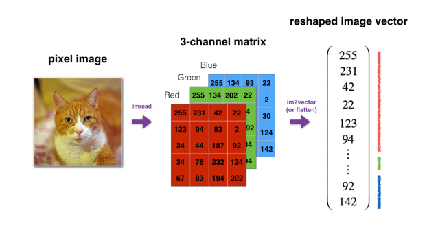
For example, in computer science, an image is represented by a 3D array of shape ( l e n g t h , h e i g h t , d e p t h = 3 ) (length, height, depth = 3) (length,height,depth=3). However, when you read an image as the input of an algorithm you convert it to a vector of shape ( l e n g t h ∗ h e i g h t ∗ 3 , 1 ) (length*height*3, 1) (length∗height∗3,1). In other words, you “unroll”, or reshape, the 3D array into a 1D vector.
Exercise: Implement image2vector() that takes an input of shape (length, height, 3) and returns a vector of shape (length*height*3, 1). For example, if you would like to reshape an array v of shape (a, b, c) into a vector of shape (a*b,c) you would do:
v = v.reshape((v.shape[0]*v.shape[1], v.shape[2])) # v.shape[0] = a ; v.shape[1] = b ; v.shape[2] = c
- Please don’t hardcode the dimensions of image as a constant. Instead look up the quantities you need with
image.shape[0], etc.
1.3 - 重塑数组形状
在深度学习中两个常用的 numpy 函数是 np.shape 和 np.reshape().
- X.shape 被用于获取矩阵/向量 X 的形状 (维度).
- X.reshape(…) 被用于将 X 重塑为其他形状 .
例如, 在计算机科学中, 一个图像可以用一个形状为 ( l e n g t h , h e i g h t , d e p t h = 3 ) (length, height, depth = 3) (length,height,depth=3) 的3维数组表示. 然而, 当你读取图像作为算法的输入,你把它转变为一个 ( l e n g t h ∗ h e i g h t ∗ 3 , 1 ) (length*height*3, 1) (length∗height∗3,1) 的向量. 换句话说, 你 “摊开”, 或者重塑这个3维数组为1维向量.

练习: 实现 image2vector() ,输入形状 (length, height, 3) 返回一个向量形状为 (length*height*3, 1). 例如,如果你想重塑一个形状为(a, b, c)的数组 v 为一个形状为(a*b,c) 的向量,你可以这样做:
v = v.reshape((v.shape[0]*v.shape[1], v.shape[2])) # v.shape[0] = a ; v.shape[1] = b ; v.shape[2] = c
- 请不要硬编码图像的维度为一个常量. 而是用
image.shape[0]获取你需要的值, 等等.
# GRADED FUNCTION: image2vector
def image2vector(image):
    """
    Argument:
    image -- a numpy array of shape (length, height, depth)

    Returns:
    v -- a vector of shape (length*height*depth, 1)
    """

    ### START CODE HERE ### (≈ 1 line of code)
    v=image.reshape((image.shape[0]*image.shape[1]*image.shape[2],1))
    ### END CODE HERE ###

    return v
# This is a 3 by 3 by 2 array, typically images will be (num_px_x, num_px_y,3) where 3 represents the RGB values
image = np.array([[[ 0.67826139,  0.29380381],
        [ 0.90714982,  0.52835647],
        [ 0.4215251 ,  0.45017551]],

       [[ 0.92814219,  0.96677647],
        [ 0.85304703,  0.52351845],
        [ 0.19981397,  0.27417313]],

       [[ 0.60659855,  0.00533165],
        [ 0.10820313,  0.49978937],
        [ 0.34144279,  0.94630077]]])

print ("image2vector(image) = " + str(image2vector(image)))
Expected Output:
| **image2vector(image)** | [[ 0.67826139] [ 0.29380381] [ 0.90714982] [ 0.52835647] [ 0.4215251 ] [ 0.45017551] [ 0.92814219] [ 0.96677647] [ 0.85304703] [ 0.52351845] [ 0.19981397] [ 0.27417313] [ 0.60659855] [ 0.00533165] [ 0.10820313] [ 0.49978937] [ 0.34144279] [ 0.94630077]] |
1.4 - Normalizing rows
Another common technique we use in Machine Learning and Deep Learning is to normalize our data. It often leads to a better performance because gradient descent converges faster after normalization. Here, by normalization we mean changing x to $ \frac{x}{| x|} $ (dividing each row vector of x by its norm).
For example, if x = [ 0 3 4 2 6 4 ] (3) x = \begin{bmatrix} 0 & 3 & 4 \\ 2 & 6 & 4 \\ \end{bmatrix}\tag{3} x=[023644](3) then ∥ x ∥ = n p . l i n a l g . n o r m ( x , a x i s = 1 , k e e p d i m s = T r u e ) = [ 5 56 ] (4) \| x\| = np.linalg.norm(x, axis = 1, keepdims = True) = \begin{bmatrix} 5 \\ \sqrt{56} \\ \end{bmatrix}\tag{4} ∥x∥=np.linalg.norm(x,axis=1,keepdims=True)=[556](4)and x _ n o r m a l i z e d = x ∥ x ∥ = [ 0 3 5 4 5 2 56 6 56 4 56 ] (5) x\_normalized = \frac{x}{\| x\|} = \begin{bmatrix} 0 & \frac{3}{5} & \frac{4}{5} \\ \frac{2}{\sqrt{56}} & \frac{6}{\sqrt{56}} & \frac{4}{\sqrt{56}} \\ \end{bmatrix}\tag{5} x_normalized=∥x∥x=[05625356654564](5) Note that you can divide matrices of different sizes and it works fine: this is called broadcasting and you’re going to learn about it in part 5.
Exercise: Implement normalizeRows() to normalize the rows of a matrix. After applying this function to an input matrix x, each row of x should be a vector of unit length (meaning length 1).
1.4 - 行标准化
我们在机器学习和深度学习中使用的另一种常见技术是标准化我们的数据. 因为梯度下降在标准化后会收敛的更快,所以这常常会有更好的效果. 这里, 标准化意味着将 x 转变为 $ \frac{x}{| x|} $ (将x的每个行向量除以其范数).
例如, 如果 x = [ 0 3 4 2 6 4 ] (3) x = \begin{bmatrix} 0 & 3 & 4 \\ 2 & 6 & 4 \\ \end{bmatrix}\tag{3} x=[023644](3) 然后 ∥ x ∥ = n p . l i n a l g . n o r m ( x , a x i s = 1 , k e e p d i m s = T r u e ) = [ 5 56 ] (4) \| x\| = np.linalg.norm(x, axis = 1, keepdims = True) = \begin{bmatrix} 5 \\ \sqrt{56} \\ \end{bmatrix}\tag{4} ∥x∥=np.linalg.norm(x,axis=1,keepdims=True)=[556](4)并且 x _ n o r m a l i z e d = x ∥ x ∥ = [ 0 3 5 4 5 2 56 6 56 4 56 ] (5) x\_normalized = \frac{x}{\| x\|} = \begin{bmatrix} 0 & \frac{3}{5} & \frac{4}{5} \\ \frac{2}{\sqrt{56}} & \frac{6}{\sqrt{56}} & \frac{4}{\sqrt{56}} \\ \end{bmatrix}\tag{5} x_normalized=∥x∥x=[05625356654564](5) 注意你可以除以不同形状的矩阵: 这叫做广播,你将在第5部分中学习.
练习: 实现 normalizeRows() 来标准化矩阵的行. 将此函数应用于输入矩阵 x,返回的 x 每一行应该是一个单位(长度为 1)向量 .
# GRADED FUNCTION: normalizeRows

def normalizeRows(x):
    """
    Implement a function that normalizes each row of the matrix x (to have unit length).

    Argument:
    x -- A numpy matrix of shape (n, m)

    Returns:
    x -- The normalized (by row) numpy matrix. You are allowed to modify x.
    """

    ### START CODE HERE ### (≈ 2 lines of code)
    # Compute x_norm as the norm 2 of x. Use np.linalg.norm(..., ord = 2, axis = ..., keepdims = True)
    x_norm=np.linalg.norm(x,axis=1,keepdims=True)
    # Divide x by its norm.
    x=x/x_norm
    ### END CODE HERE ###

    return x
x = np.array([
    [0, 3, 4],
    [1, 6, 4]])
print("normalizeRows(x) = " + str(normalizeRows(x)))
Expected Output:
| **normalizeRows(x)** | [[ 0. 0.6 0.8 ] [ 0.13736056 0.82416338 0.54944226]] |
Note:
In normalizeRows(), you can try to print the shapes of x_norm and x, and then rerun the assessment. You’ll find out that they have different shapes. This is normal given that x_norm takes the norm of each row of x. So x_norm has the same number of rows but only 1 column. So how did it work when you divided x by x_norm? This is called broadcasting and we’ll talk about it now!
注意:
在 normalizeRows() 中, 你可以尝试输出 x_norm 和 x 的尺寸, 然后重新运行.你会发现他们有不同的尺寸.这是正常的, x_norm 是 x 每一行的范数. 所以 x_norm 有相同的行数,但是它只有 1 列. 那么当 x 除以 x_norm 时是如何执行的? 这叫做广播,我们现在就讨论它!
1.5 - Broadcasting and the softmax function
A very important concept to understand in numpy is “broadcasting”. It is very useful for performing mathematical operations between arrays of different shapes. For the full details on broadcasting, you can read the official broadcasting documentation.
1.5 -广播和 softmax 函数
“广播” 是numpy中一个非常重要的概念. 对于在不同形状的数组之间执行数学运算非常有用. 广播的更多细节, 你可以阅读官方 广播文档.
Exercise: Implement a softmax function using numpy. You can think of softmax as a normalizing function used when your algorithm needs to classify two or more classes. You will learn more about softmax in the second course of this specialization.
Instructions:
练习:使用 numpy 实现一个 softmax 函数. 当你的算法需要两个或多个分类的时候,你可以把 softmax 想象为一个标准化函数. 在本专业的第二门课中,你将学到更多关于 softmax 的知识.
要求:
# GRADED FUNCTION: softmax
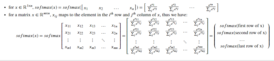
def softmax(x):
"""Calculates the softmax for each row of the input x.
Your code should work for a row vector and also for matrices of shape (n, m).
Argument:
x -- A numpy matrix of shape (n,m)
Returns:
s -- A numpy matrix equal to the softmax of x, of shape (n,m)
"""
### START CODE HERE ### (≈ 3 lines of code)
# Apply exp() element-wise to x. Use np.exp(...).
x_exp=np.exp(x)
# Create a vector x_sum that sums each row of x_exp. Use np.sum(..., axis = 1, keepdims = True).
x_sum=np.sum(x_exp,axis=1,keepdims=True)
# Compute softmax(x) by dividing x_exp by x_sum. It should automatically use numpy broadcasting.
s=x_exp/x_sum
### END CODE HERE ###
return s
x = np.array([
    [9, 2, 5, 0, 0],
    [7, 5, 0, 0 ,0]])
print("softmax(x) = " + str(softmax(x)))
Expected Output:
| **softmax(x)** | [[ 9.80897665e-01 8.94462891e-04 1.79657674e-02 1.21052389e-04 1.21052389e-04] [ 8.78679856e-01 1.18916387e-01 8.01252314e-04 8.01252314e-04 8.01252314e-04]] |
Note:
- If you print the shapes of x_exp, x_sum and s above and rerun the assessment cell, you will see that x_sum is of shape (2,1) while x_exp and s are of shape (2,5). x_exp/x_sum works due to python broadcasting.
Congratulations! You now have a pretty good understanding of python numpy and have implemented a few useful functions that you will be using in deep learning.
注意:
- 如果你打印 x_exp, x_sum 和 s 的形状, 你会发现 x_sum 的形状为 (2,1) 但 x_exp 和 s 的形状 (2,5). x_exp/x_sum 能运行是因为python的广播.
恭喜! 你现在已经很好的理解了 python 的 numpy 并且实现了一些在深度学习中很有用的函数.
What you need to remember:
- np.exp(x) works for any np.array x and applies the exponential function to every coordinate
- the sigmoid function and its gradient
- image2vector is commonly used in deep learning
- np.reshape is widely used. In the future, you’ll see that keeping your matrix/vector dimensions straight will go toward eliminating a lot of bugs.
- numpy has efficient built-in functions
- broadcasting is extremely useful
你需要记住:
- np.exp(x) 适用于任何 np.array x 并且计算每一个的指数
- sigmoid 函数和它的梯度
- image2vector 在深度学习中很常用
- np.reshape 使用广泛. 在未来, 你会看到保持矩阵/向量的的维度不变会避免很多bug.
- numpy 具有高效的内置函数
- 广播非常有用
2) Vectorization(向量化)
In deep learning, you deal with very large datasets. Hence, a non-computationally-optimal function can become a huge bottleneck in your algorithm and can result in a model that takes ages to run. To make sure that your code is computationally efficient, you will use vectorization. For example, try to tell the difference between the following implementations of the dot/outer/elementwise product.
在深度学习中, 你需要处理非常大的数据集. 然而, 一个非计算最优的函数可能会成为你的算法中的一个巨大瓶颈并且导致模型需要很长运行时间.为了使你的代码计算更高效,你将使用向量化. 例如, 尝试区分以下 点积/外积/元素乘法 实现之间的区别.
import time

x1 = [9, 2, 5, 0, 0, 7, 5, 0, 0, 0, 9, 2, 5, 0, 0]
x2 = [9, 2, 2, 9, 0, 9, 2, 5, 0, 0, 9, 2, 5, 0, 0]

### CLASSIC DOT PRODUCT OF VECTORS IMPLEMENTATION ###
tic = time.process_time()
dot = 0
for i in range(len(x1)):
    dot+= x1[i]*x2[i]
toc = time.process_time()
print ("dot = " + str(dot) + "\n ----- Computation time = " + str(1000*(toc - tic)) + "ms")

### CLASSIC OUTER PRODUCT IMPLEMENTATION ###
tic = time.process_time()
outer = np.zeros((len(x1),len(x2))) # we create a len(x1)*len(x2) matrix with only zeros
for i in range(len(x1)):
    for j in range(len(x2)):
        outer[i,j] = x1[i]*x2[j]
toc = time.process_time()
print ("outer = " + str(outer) + "\n ----- Computation time = " + str(1000*(toc - tic)) + "ms")

### CLASSIC ELEMENTWISE IMPLEMENTATION ###
tic = time.process_time()
mul = np.zeros(len(x1))
for i in range(len(x1)):
    mul[i] = x1[i]*x2[i]
toc = time.process_time()
print ("elementwise multiplication = " + str(mul) + "\n ----- Computation time = " + str(1000*(toc - tic)) + "ms")

### CLASSIC GENERAL DOT PRODUCT IMPLEMENTATION ###
W = np.random.rand(3,len(x1)) # Random 3*len(x1) numpy array
tic = time.process_time()
gdot = np.zeros(W.shape[0])
for i in range(W.shape[0]):
    for j in range(len(x1)):
        gdot[i] += W[i,j]*x1[j]
toc = time.process_time()
print ("gdot = " + str(gdot) + "\n ----- Computation time = " + str(1000*(toc - tic)) + "ms")
x1 = [9, 2, 5, 0, 0, 7, 5, 0, 0, 0, 9, 2, 5, 0, 0]
x2 = [9, 2, 2, 9, 0, 9, 2, 5, 0, 0, 9, 2, 5, 0, 0]

### VECTORIZED DOT PRODUCT OF VECTORS ###
tic = time.process_time()
dot = np.dot(x1,x2)
toc = time.process_time()
print ("dot = " + str(dot) + "\n ----- Computation time = " + str(1000*(toc - tic)) + "ms")

### VECTORIZED OUTER PRODUCT ###
tic = time.process_time()
outer = np.outer(x1,x2)
toc = time.process_time()
print ("outer = " + str(outer) + "\n ----- Computation time = " + str(1000*(toc - tic)) + "ms")

### VECTORIZED ELEMENTWISE MULTIPLICATION ###
tic = time.process_time()
mul = np.multiply(x1,x2)
toc = time.process_time()
print ("elementwise multiplication = " + str(mul) + "\n ----- Computation time = " + str(1000*(toc - tic)) + "ms")

### VECTORIZED GENERAL DOT PRODUCT ###
tic = time.process_time()
dot = np.dot(W,x1)
toc = time.process_time()
print ("gdot = " + str(dot) + "\n ----- Computation time = " + str(1000*(toc - tic)) + "ms")
As you may have noticed, the vectorized implementation is much cleaner and more efficient. For bigger vectors/matrices, the differences in running time become even bigger.
Note that np.dot() performs a matrix-matrix or matrix-vector multiplication. This is different from np.multiply() and the * operator (which is equivalent to .* in Matlab/Octave), which performs an element-wise multiplication.
你可能注意到, 向量化的实现更清晰并且更高效. 对于更大的向量/矩阵, 运行时间差异会更大.
注意 np.dot() 执行的是 矩阵-矩阵 或 矩阵-向量 的乘法. 这与 np.multiply() 和 * 操作 (相同于Matlab/Octave中的 .* )不同, 这表示元素乘法.
2.1 Implement the L1 and L2 loss functions
Exercise: Implement the numpy vectorized version of the L1 loss. You may find the function abs(x) (absolute value of x) useful.
Reminder:
- The loss is used to evaluate the performance of your model. The bigger your loss is, the more different your predictions ($ \hat{y} ) a r e f r o m t h e t r u e v a l u e s ( ) are from the true values ( )arefromthetruevalues(y$). In deep learning, you use optimization algorithms like Gradient Descent to train your model and to minimize the cost.
- L1 loss is defined as:
L 1 ( y ^ , y ) = ∑ i = 0 m ∣ y ( i ) − y ^ ( i ) ∣ (6) \begin{aligned} & L_1(\hat{y}, y) = \sum_{i=0}^m|y^{(i)} - \hat{y}^{(i)}| \end{aligned}\tag{6} L1(y^,y)=i=0∑m∣y(i)−y^(i)∣(6)
2.1 实现 L1 和 L2 损失函数
练习: 实现 numpy 向量化版本的 L1 损失. 你可能会发现 abs(x) (x 的绝对值)函数很有用.
提醒:
- 损失用于评价你模型的性能. 损失越大, 你的预测 ($ \hat{y} ) 和 真 实 值 ( ) 和真实值 ( )和真实值(y$) 差异越大. 在深度学习中, 使用优化算法例如梯度下降来训练模型并最小化损失.
- L1 损失定义如下:
L 1 ( y ^ , y ) = ∑ i = 0 m ∣ y ( i ) − y ^ ( i ) ∣ (6) \begin{aligned} & L_1(\hat{y}, y) = \sum_{i=0}^m|y^{(i)} - \hat{y}^{(i)}| \end{aligned}\tag{6} L1(y^,y)=i=0∑m∣y(i)−y^(i)∣(6)
# GRADED FUNCTION: L1

def L1(yhat, y):
    """
    Arguments:
    yhat -- vector of size m (predicted labels)
    y -- vector of size m (true labels)

    Returns:
    loss -- the value of the L1 loss function defined above
    """

    ### START CODE HERE ### (≈ 1 line of code)
    loss=np.sum(np.abs(yhat-y))
    ### END CODE HERE ###

    return loss
yhat = np.array([.9, 0.2, 0.1, .4, .9])
y = np.array([1, 0, 0, 1, 1])
print("L1 = " + str(L1(yhat,y)))
Expected Output:
| **L1** | 1.1 |
Exercise: Implement the numpy vectorized version of the L2 loss. There are several way of implementing the L2 loss but you may find the function np.dot() useful. As a reminder, if
x
=
[
x
1
,
x
2
,
.
.
.
,
x
n
]
x = [x_1, x_2, ..., x_n]
x=[x1,x2,...,xn], then np.dot(x,x) =
∑
j
=
0
n
x
j
2
\sum_{j=0}^n x_j^{2}
∑j=0nxj2.
- L2 loss is defined as L 2 ( y ^ , y ) = ∑ i = 0 m ( y ( i ) − y ^ ( i ) ) 2 (7) \begin{aligned} & L_2(\hat{y},y) = \sum_{i=0}^m(y^{(i)} - \hat{y}^{(i)})^2 \end{aligned}\tag{7} L2(y^,y)=i=0∑m(y(i)−y^(i))2(7)
练习: 实现 numpy 向量化版本的 L2 损失. 有很多方法实现 L2 损失,但是你会发现 np.dot()函数很有用. 提醒一下, 如果
x
=
[
x
1
,
x
2
,
.
.
.
,
x
n
]
x = [x_1, x_2, ..., x_n]
x=[x1,x2,...,xn], 则 np.dot(x,x) =
∑
j
=
0
n
x
j
2
\sum_{j=0}^n x_j^{2}
∑j=0nxj2.
- L2 损失定义 L 2 ( y ^ , y ) = ∑ i = 0 m ( y ( i ) − y ^ ( i ) ) 2 (7) \begin{aligned} & L_2(\hat{y},y) = \sum_{i=0}^m(y^{(i)} - \hat{y}^{(i)})^2 \end{aligned}\tag{7} L2(y^,y)=i=0∑m(y(i)−y^(i))2(7)
# GRADED FUNCTION: L2

def L2(yhat, y):
    """
    Arguments:
    yhat -- vector of size m (predicted labels)
    y -- vector of size m (true labels)

    Returns:
    loss -- the value of the L2 loss function defined above
    """

    ### START CODE HERE ### (≈ 1 line of code)
    loss=np.sum(np.dot(yhat-y,yhat-y))
    ### END CODE HERE ###

    return loss
yhat = np.array([.9, 0.2, 0.1, .4, .9])
y = np.array([1, 0, 0, 1, 1])
print("L2 = " + str(L2(yhat,y)))
Expected Output:
| **L2** | 0.43 |
Congratulations on completing this assignment. We hope that this little warm-up exercise helps you in the future assignments, which will be more exciting and interesting!
祝贺你完成了作业. 希望这个热身练习能在未来的作业中帮助你, 这样会更刺激更有趣!
What to remember:
- Vectorization is very important in deep learning. It provides computational efficiency and clarity.
- You have reviewed the L1 and L2 loss.
- You are familiar with many numpy functions such as np.sum, np.dot, np.multiply, np.maximum, etc…
记住:
- 向量化在深度学习中很重要.它使计算更高效更清楚.
- 复习了 L1 和 L2 损失.
- 熟悉了很多 numpy 函数例如 np.sum, np.dot, np.multiply, np.maximum, 等等…


 359
359


 被折叠的 条评论
为什么被折叠?
被折叠的 条评论
为什么被折叠?
 到【灌水乐园】发言


