


卷积神经网络(Convolutional Neural Network,CNN)
- 受生物学上感受野机制的启发而提出。
- 一般是由卷积层、汇聚层和全连接层交叉堆叠而成的前馈神经网络
- 有三个结构上的特性:局部连接、权重共享、汇聚。
具有一定程度上的平移、缩放和旋转不变性。 - 和前馈神经网络相比,卷积神经网络的参数更少。
- 主要应用在图像和视频分析的任务上,其准确率一般也远远超出了其他的神经网络模型。
- 近年来卷积神经网络也广泛地应用到自然语言处理、推荐系统等领域。
5.1 卷积
考虑到使用全连接前馈网络来处理图像时,会出现如下问题:
模型参数过多,容易发生过拟合。 在全连接前馈网络中,隐藏层的每个神经元都要跟该层所有输入的神经元相连接。随着隐藏层神经元数量的增多,参数的规模也会急剧增加,导致整个神经网络的训练效率非常低,也很容易发生过拟合。
难以提取图像中的局部不变性特征。 自然图像中的物体都具有局部不变性特征,比如尺度缩放、平移、旋转等操作不影响其语义信息。而全连接前馈网络很难提取这些局部不变性特征。
卷积神经网络有三个结构上的特性:局部连接、权重共享和汇聚。这些特性使得卷积神经网络具有一定程度上的平移、缩放和旋转不变性。和前馈神经网络相比,卷积神经网络的参数也更少。因此,通常会使用卷积神经网络来处理图像信息。
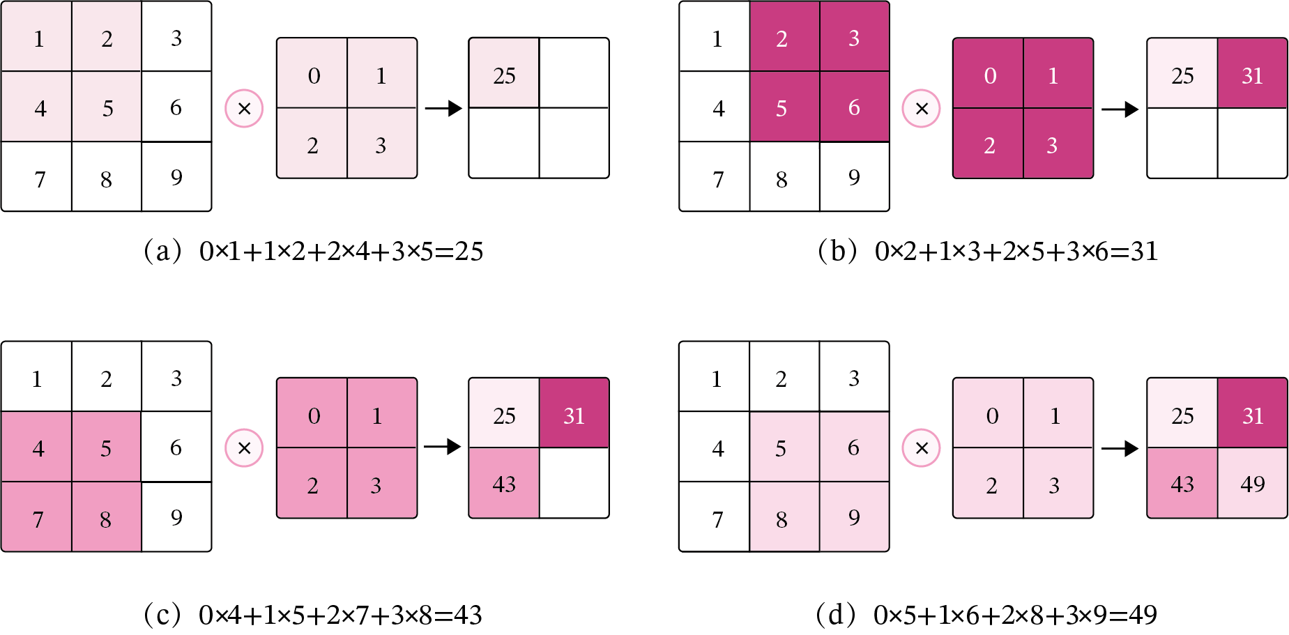
5.1.1 二维卷积运算
在机器学习和图像处理领域,卷积的主要功能是在一个图像(或特征图)上滑动一个卷积核,通过卷积操作得到一组新的特征。在计算卷积的过程中,需要进行卷积核的翻转,而这也会带来一些不必要的操作和开销。因此,在具体实现上,一般会以数学中的互相关(Cross-Correlatio)运算来代替卷积。 在神经网络中,卷积运算的主要作用是抽取特征,卷积核是否进行翻转并不会影响其特征抽取的能力。特别是当卷积核是可学习的参数时,卷积和互相关在能力上是等价的。因此,很多时候,为方便起见,会直接用互相关来代替卷积。
以发现,使用卷积处理图像,会有以下两个特性:
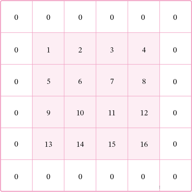
在卷积层(假设是第 𝑙 层)中的每一个神经元都只和前一层(第 𝑙−1 层)中某个局部窗口内的神经元相连,构成一个局部连接网络,这也就是卷积神经网络的局部连接特性。
由于卷积的主要功能是在一个图像(或特征图)上滑动一个卷积核,所以作为参数的卷积核 𝐖∈ℝ𝑈×𝑉 对于第 𝑙 层的所有的神经元都是相同的,这也就是卷积神经网络的权重共享特性。
5.1.2 二维卷积算子
【使用pytorch实现】
在本书后面的实现中,算子都继承torch.nn.Layer,并使用反向传播进行实现。
import torch#导入包
class Conv2D(torch.nn.Module):#继承torch.nn.Module下的二维卷积算子
def __init__(self, kernel_size, weight_attr=torch.tensor([[0., 1.],[2., 3.]])):#类初始化,初始化权重属性为默认值
super(Conv2D, self).__init__()#继承torch.nn.Module中的Conv2D卷积算子
self.weight = torch.nn.Parameter(weight_attr)
#torch.nn.Parameter将一个不可训练的类型为Tensor的参数转化为可训练的类型为parameter的参数,并将这个参数绑定到module里面,成为module中可训练的参数。
self.weight.reshape([kernel_size,kernel_size])#将卷积核大小改为kernel_size*kernel_size
def forward(self, X):#定义前向传播
"""
输入:
- X:输入矩阵,shape=[B, M, N],B为样本数量
输出:
- output:输出矩阵
"""
u, v = self.weight.shape#得到输入形状大小
output = torch.zeros([X.shape[0], X.shape[1] - u + 1, X.shape[2] - v + 1])#初始化输出矩阵
for i in range(output.shape[1]):
for j in range(output.shape[2]):
output[:, i, j] = torch.sum(X[:, i:i+u, j:j+v]*self.weight, axis=[1,2])#进行卷积
return output
# 随机构造一个二维输入矩阵
torch.manual_seed(100)#定义随机种子
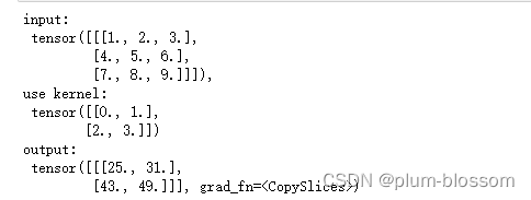
inputs = torch.tensor([[[1.,2.,3.],[4.,5.,6.],[7.,8.,9.]]])#初始化输入
kernel = torch.tensor([[0.,1.],[2.,3.]])#初始化kernel即weight_attr
conv2d = Conv2D(kernel_size=2)#传入kernel_size参数
outputs = conv2d(inputs)#测试二维卷积算子
print("input:\n {}, \nuse kernel:\n {}\noutput:\n {}".format(inputs,kernel, outputs))#输出结果。
运行结果:
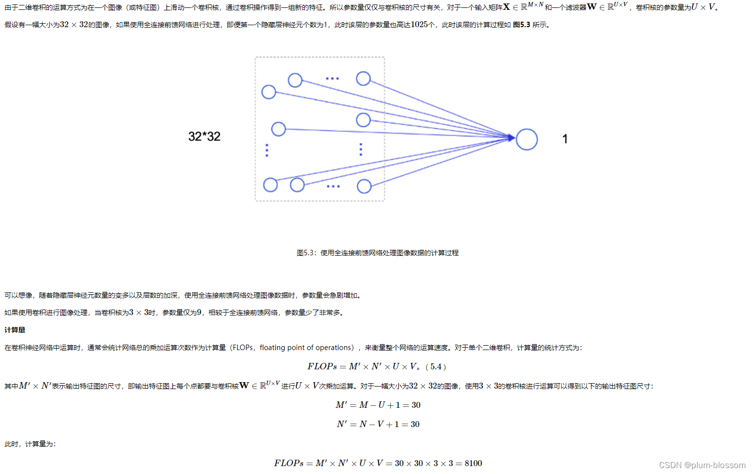
5.1.3 二维卷积的参数量和计算量
随着隐藏层神经元数量的变多以及层数的加深,
使用全连接前馈网络处理图像数据时,参数量会急剧增加。
如果使用卷积进行图像处理,相较于全连接前馈网络,参数量少了非常多。
5.1.4 感受野


5.1.5 卷积的变种
5.1.5.1 步长(Stride)
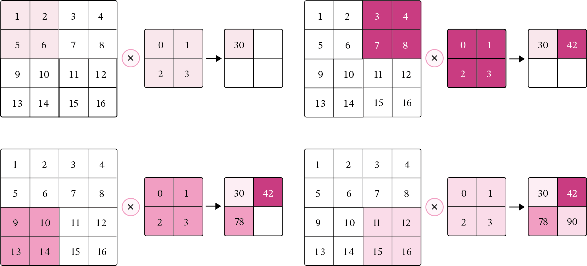
5.1.5.2 零填充(Zero Padding)
5.1.6 带步长和零填充的二维卷积算子
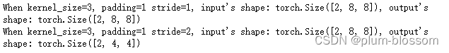
从输出结果看出,使用3×3大小卷积,
padding为1,
当stride=1时,模型的输出特征图与输入特征图保持一致;
当stride=2时,模型的输出特征图的宽和高都缩小一倍。
【使用pytorch实现】
class Conv2D(torch.nn.Module):#继承torch.nn.Module下的二维卷积算子
    def __init__(self, kernel_size, stride=1, padding=0, weight_attr=torch.ones([3,3])):
        super(Conv2D, self).__init__()
        self.weight = torch.nn.Parameter(weight_attr)
        self.weight.reshape([kernel_size,kernel_size])
        # 步长
        self.stride = stride
        # 零填充
        self.padding = padding

    def forward(self, X):
        # 零填充
        new_X = torch.zeros([X.shape[0], X.shape[1]+2*self.padding, X.shape[2]+2*self.padding])#初始化填充
        new_X[:, self.padding:X.shape[1]+self.padding, self.padding:X.shape[2]+self.padding] = X#填充
        u, v = self.weight.shape#获得形状大小
        output_w = (new_X.shape[1] - u) // self.stride + 1#计算输出width
        output_h = (new_X.shape[2] - v) // self.stride + 1#计算输出height
        output = torch.zeros([X.shape[0], output_w, output_h])#初始化输出
        for i in range(0, output.shape[1]):
            for j in range(0, output.shape[2]):
                output[:, i, j] = torch.sum(
                    new_X[:, self.stride*i:self.stride*i+u, self.stride*j:self.stride*j+v]*self.weight,#卷积
                    axis=[1,2])
        return output

inputs = torch.randn([2, 8, 8])#初始化输入大小
conv2d_padding = Conv2D(kernel_size=3, stride=1,padding=1)
outputs = conv2d_padding(inputs)
print("When kernel_size=3, padding=1 stride=1, input's shape: {}, output's shape: {}".format(inputs.shape, outputs.shape))
conv2d_stride = Conv2D(kernel_size=3, stride=2, padding=1)
outputs = conv2d_stride(inputs)
print("When kernel_size=3, padding=1 stride=2, input's shape: {}, output's shape: {}".format(inputs.shape, outputs.shape))
运行结果:
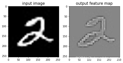
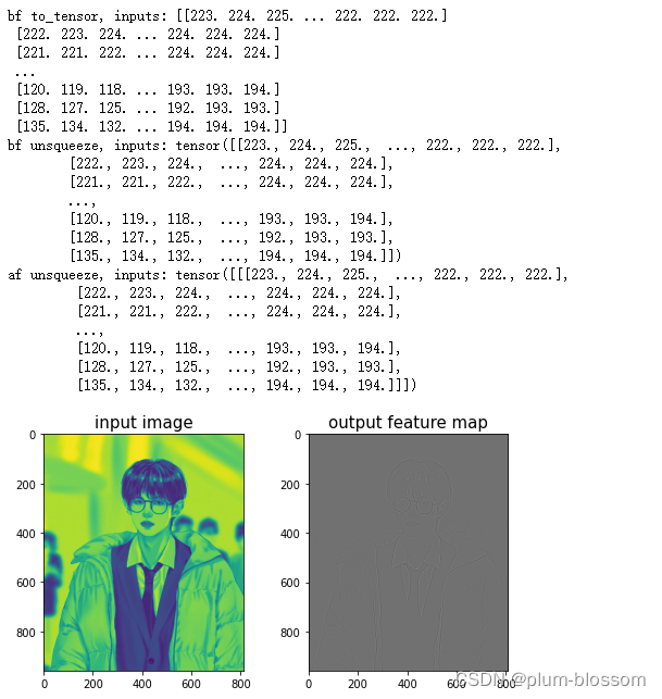
5.1.7 使用卷积运算完成图像边缘检测任务
【使用pytorch实现】
%matplotlib inline
import matplotlib.pyplot as plt
from PIL import Image
import numpy as np
# 读取图片
img = Image.open('12.jpg').convert('L')#转成灰度图
img.resize((256,256))
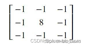
# 设置卷积核参数
w = np.array([[-1,-1,-1], [-1,8,-1], [-1,-1,-1]], dtype='float32')
# 创建卷积算子,卷积核大小为3x3,并使用上面的设置好的数值作为卷积核权重的初始化参数
conv = Conv2D(kernel_size=3, stride=1, padding=0, weight_attr=torch.tensor(w))
# 将读入的图片转化为float32类型的numpy.ndarray
inputs = np.array(img).astype('float32')
print("bf to_tensor, inputs:",inputs)
# 将图片转为Tensor
inputs = torch.tensor(inputs)
print("bf unsqueeze, inputs:",inputs)
inputs = torch.unsqueeze(inputs, axis=0)
print("af unsqueeze, inputs:",inputs)
outputs = conv(inputs)
outputs.detach().numpy()
# 可视化结果
plt.figure(figsize=(8, 4))
f = plt.subplot(121)
f.set_title('input image', fontsize=15)
plt.imshow(img)
f = plt.subplot(122)
f.set_title('output feature map', fontsize=15)
plt.imshow(outputs.detach().numpy().squeeze(), cmap='gray')
plt.savefig('conv-vis.pdf')
plt.show()
运行结果:
选做题
Pytorch实现1、2;阅读3、4、5写体会。
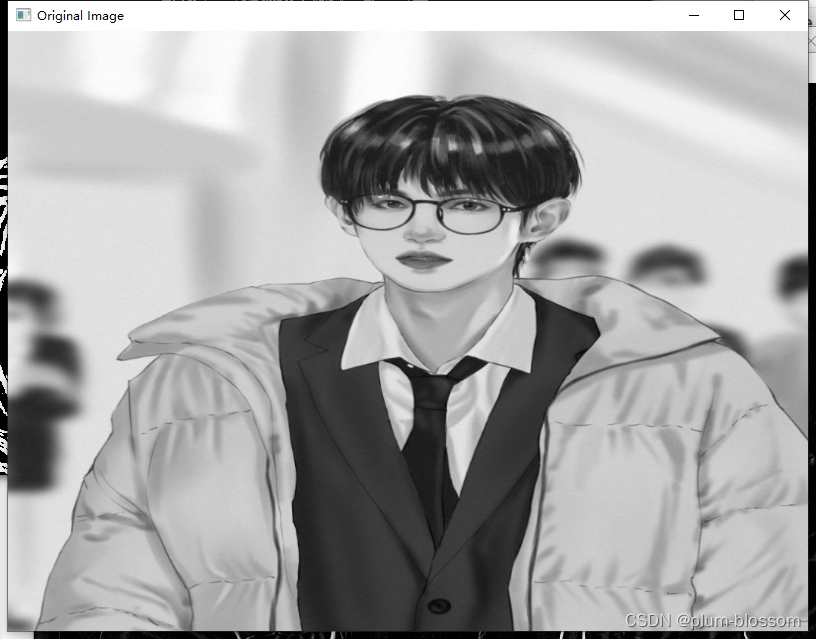
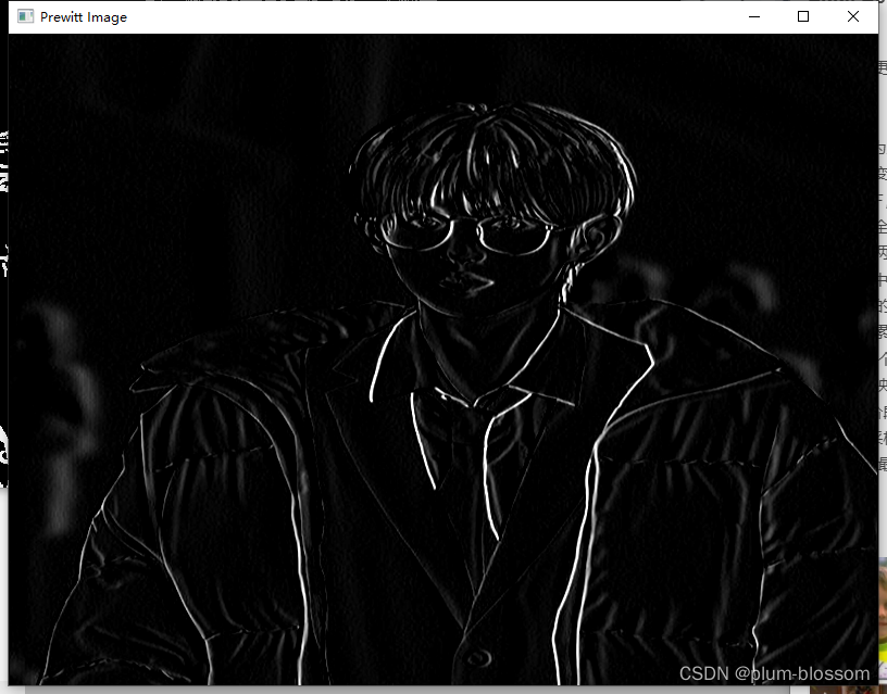
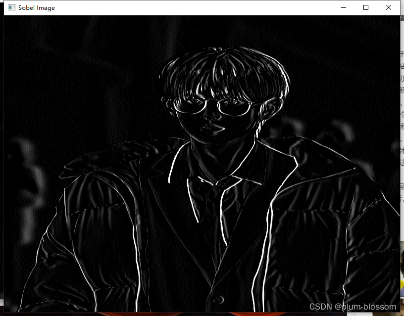
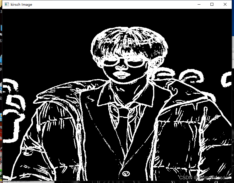
1.实现一些传统边缘检测算子,如:Roberts、Prewitt、Sobel、Scharr、Kirsch、Robinson、Laplacian
import cv2
import numpy as np

# 加载图像
image = cv2.imread('12.jpg', 0)
image = cv2.resize(image, (800, 800))
# 自定义卷积核
# Roberts边缘算子
kernel_Roberts_x = np.array([
    [1, 0],
    [0, -1]
])
kernel_Roberts_y = np.array([
    [0, -1],
    [1, 0]
])
# Sobel边缘算子
kernel_Sobel_x = np.array([
    [-1, 0, 1],
    [-2, 0, 2],
    [-1, 0, 1]])
kernel_Sobel_y = np.array([
    [1, 2, 1],
    [0, 0, 0],
    [-1, -2, -1]])
# Prewitt边缘算子
kernel_Prewitt_x = np.array([
    [-1, 0, 1],
    [-1, 0, 1],
    [-1, 0, 1]])
kernel_Prewitt_y = np.array([
    [1, 1, 1],
    [0, 0, 0],
    [-1, -1, -1]])


# Kirsch 边缘检测算子
def kirsch(image):
    m, n = image.shape
    list = []
    kirsch = np.zeros((m, n))
    for i in range(2, m - 1):
        for j in range(2, n - 1):
            d1 = np.square(5 * image[i - 1, j - 1] + 5 * image[i - 1, j] + 5 * image[i - 1, j + 1] -
                           3 * image[i, j - 1] - 3 * image[i, j + 1] - 3 * image[i + 1, j - 1] -
                           3 * image[i + 1, j] - 3 * image[i + 1, j + 1])
            d2 = np.square((-3) * image[i - 1, j - 1] + 5 * image[i - 1, j] + 5 * image[i - 1, j + 1] -
                           3 * image[i, j - 1] + 5 * image[i, j + 1] - 3 * image[i + 1, j - 1] -
                           3 * image[i + 1, j] - 3 * image[i + 1, j + 1])
            d3 = np.square((-3) * image[i - 1, j - 1] - 3 * image[i - 1, j] + 5 * image[i - 1, j + 1] -
                           3 * image[i, j - 1] + 5 * image[i, j + 1] - 3 * image[i + 1, j - 1] -
                           3 * image[i + 1, j] + 5 * image[i + 1, j + 1])
            d4 = np.square((-3) * image[i - 1, j - 1] - 3 * image[i - 1, j] - 3 * image[i - 1, j + 1] -
                           3 * image[i, j - 1] + 5 * image[i, j + 1] - 3 * image[i + 1, j - 1] +
                           5 * image[i + 1, j] + 5 * image[i + 1, j + 1])
            d5 = np.square((-3) * image[i - 1, j - 1] - 3 * image[i - 1, j] - 3 * image[i - 1, j + 1] - 3
                           * image[i, j - 1] - 3 * image[i, j + 1] + 5 * image[i + 1, j - 1] +
                           5 * image[i + 1, j] + 5 * image[i + 1, j + 1])
            d6 = np.square((-3) * image[i - 1, j - 1] - 3 * image[i - 1, j] - 3 * image[i - 1, j + 1] +
                           5 * image[i, j - 1] - 3 * image[i, j + 1] + 5 * image[i + 1, j - 1] +
                           5 * image[i + 1, j] - 3 * image[i + 1, j + 1])
            d7 = np.square(5 * image[i - 1, j - 1] - 3 * image[i - 1, j] - 3 * image[i - 1, j + 1] +
                           5 * image[i, j - 1] - 3 * image[i, j + 1] + 5 * image[i + 1, j - 1] -
                           3 * image[i + 1, j] - 3 * image[i + 1, j + 1])
            d8 = np.square(5 * image[i - 1, j - 1] + 5 * image[i - 1, j] - 3 * image[i - 1, j + 1] +
                           5 * image[i, j - 1] - 3 * image[i, j + 1] - 3 * image[i + 1, j - 1] -
                           3 * image[i + 1, j] - 3 * image[i + 1, j + 1])

            # 第一种方法:取各个方向的最大值,效果并不好,采用另一种方法
            list = [d1, d2, d3, d4, d5, d6, d7, d8]
            kirsch[i, j] = int(np.sqrt(max(list)))
    for i in range(m):
        for j in range(n):
            if kirsch[i, j] > 127:
                kirsch[i, j] = 255
            else:
                kirsch[i, j] = 0
    return kirsch


# 拉普拉斯卷积核
kernel_Laplacian_1 = np.array([
    [0, 1, 0],
    [1, -4, 1],
    [0, 1, 0]])
kernel_Laplacian_2 = np.array([
    [1, 1, 1],
    [1, -8, 1],
    [1, 1, 1]])
# 下面两个卷积核不具有旋转不变性
kernel_Laplacian_3 = np.array([
    [2, -1, 2],
    [-1, -4, -1],
    [2, 1, 2]])
kernel_Laplacian_4 = np.array([
    [-1, 2, -1],
    [2, -4, 2],
    [-1, 2, -1]])
# 5*5 LoG卷积模板
kernel_LoG = np.array([
    [0, 0, -1, 0, 0],
    [0, -1, -2, -1, 0],
    [-1, -2, 16, -2, -1],
    [0, -1, -2, -1, 0],
    [0, 0, -1, 0, 0]])
# 卷积
output_1 = cv2.filter2D(image, -1, kernel_Prewitt_x)
output_2 = cv2.filter2D(image, -1, kernel_Sobel_x)
output_3 = cv2.filter2D(image, -1, kernel_Prewitt_x)
output_4 = cv2.filter2D(image, -1, kernel_Laplacian_1)
output_5 = kirsch(image)
# 显示锐化效果
image = cv2.resize(image, (800, 600))
output_1 = cv2.resize(output_1, (800, 600))
output_2 = cv2.resize(output_2, (800, 600))
output_3 = cv2.resize(output_3, (800, 600))
output_4 = cv2.resize(output_4, (800, 600))
output_5 = cv2.resize(output_5, (800, 600))
cv2.imshow('Original Image', image)
cv2.imshow('Prewitt Image', output_1)
cv2.imshow('Sobel Image', output_2)
cv2.imshow('Prewitt Image', output_3)
cv2.imshow('Laplacian Image', output_4)
cv2.imshow('kirsch Image', output_5)
# 停顿
if cv2.waitKey(0) & 0xFF == 27:
    cv2.destroyAllWindows()
运行结果:

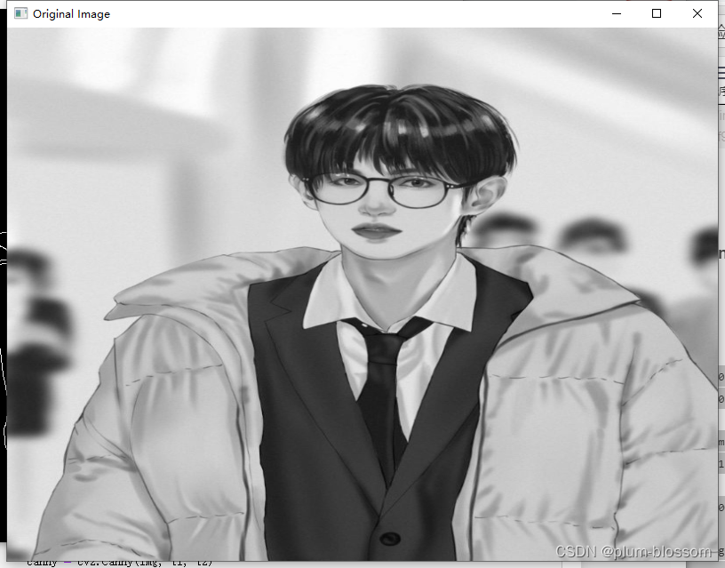
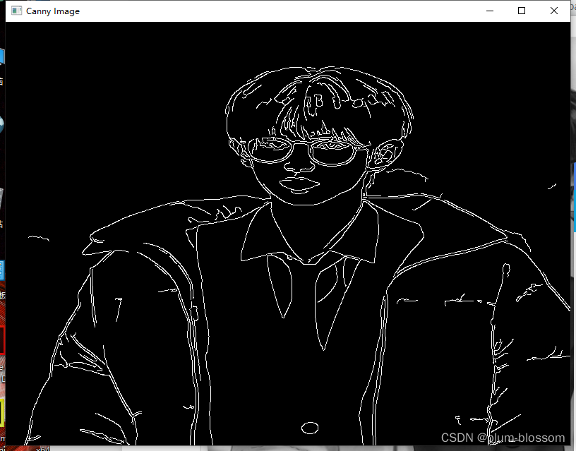
2.实现的简易的 Canny 边缘检测算法
import cv2
# 加载图像
image = cv2.imread('12.jpg',0)
image = cv2.resize(image,(800,800))
def Canny(image,k,t1,t2):
    img = cv2.GaussianBlur(image, (k, k), 0)
    canny = cv2.Canny(img, t1, t2)
    return canny
image = cv2.resize(image, (800, 600))
cv2.imshow('Original Image', image)
output =cv2.resize(Canny(image,3,50,150),(800,600))
cv2.imshow('Canny Image', output)
# 停顿
if cv2.waitKey(0) & 0xFF == 27:
    cv2.destroyAllWindows()
运行结果:
3.复现论文 Holistically-Nested Edge Detection,发表于 CVPR 2015
论文地址: https://arxiv.org/pdf/1504.06375.pdf
HED通过深度学习网络实现边缘检测,网络主要有以下两个特点
Holistically:指端到端(end-to-end 或者image-to-image)的学习方式,也就是说,网络的输入为原图,输出为边缘检测得到的二值化图像。
Nested:意思是嵌套的。在论文中指,在每层卷积层后输出该层的结果(responses produced at hidden layers ),这个结果在论文中称为side outputs。不同隐藏层的Side output尺度不同,而且,HED不止要求最后输出的边缘图像好,也要求各side output的结果要好,即学习对象是最终的输出和各Side outputs

网络结构:

HED是在VGG网络基础上改造的,卷积层后添加side output。网络层次越深,卷积核越大,side output越小,最终的输出是对多个side output特征的融合。图1中粗虚线路径被称为Deep supervision(或者说hidden layer supervision)。细虚线路径称为weight-fusion supervision。下图3为VGG16网络结构。图3中每个颜色是一个Stage,HED去掉了最后一个池化层及后面的FC层(即论文中所说的FCN–fully convolutional neural networks),保留了前面5个stage,每个stage的最后一个conv后添加一个side output。Side output层的卷积核大小为1*1,通道数与每阶段最后一层conv的通道数相同。也就是说每个side output的输出通道数为1。至于说不同大小的Side output怎么融合为输出—答案是会进行反卷积或者说进行双线性插值(反卷积理论上可拟合任何插值函数,Bilinear interpolate 可理解为反卷积的一种,论文中采用bilinear)
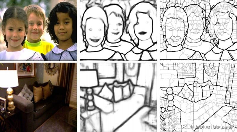
4.复现论文 Richer Convolutional Features for Edge Detection,CVPR 2017 发表
论文地址: https://arxiv.org/pdf/1612.02103v3.pdf
一个基于更丰富的卷积特征的边缘检测模型 【RCF】
RCF:
- VGG作为主干网络,每个卷积层捕获的有用信息随着感受野大小的增加而变得更粗糙(以下5条是论文中对网络架构的介绍)
- 提出RCF,切断了所有全连接层、池化层第5层,切除全连接层是为了使用全卷积层,实现image-to-image的预测,加入pool5层会使步幅增加两倍,这通常会导致边缘定位的退化
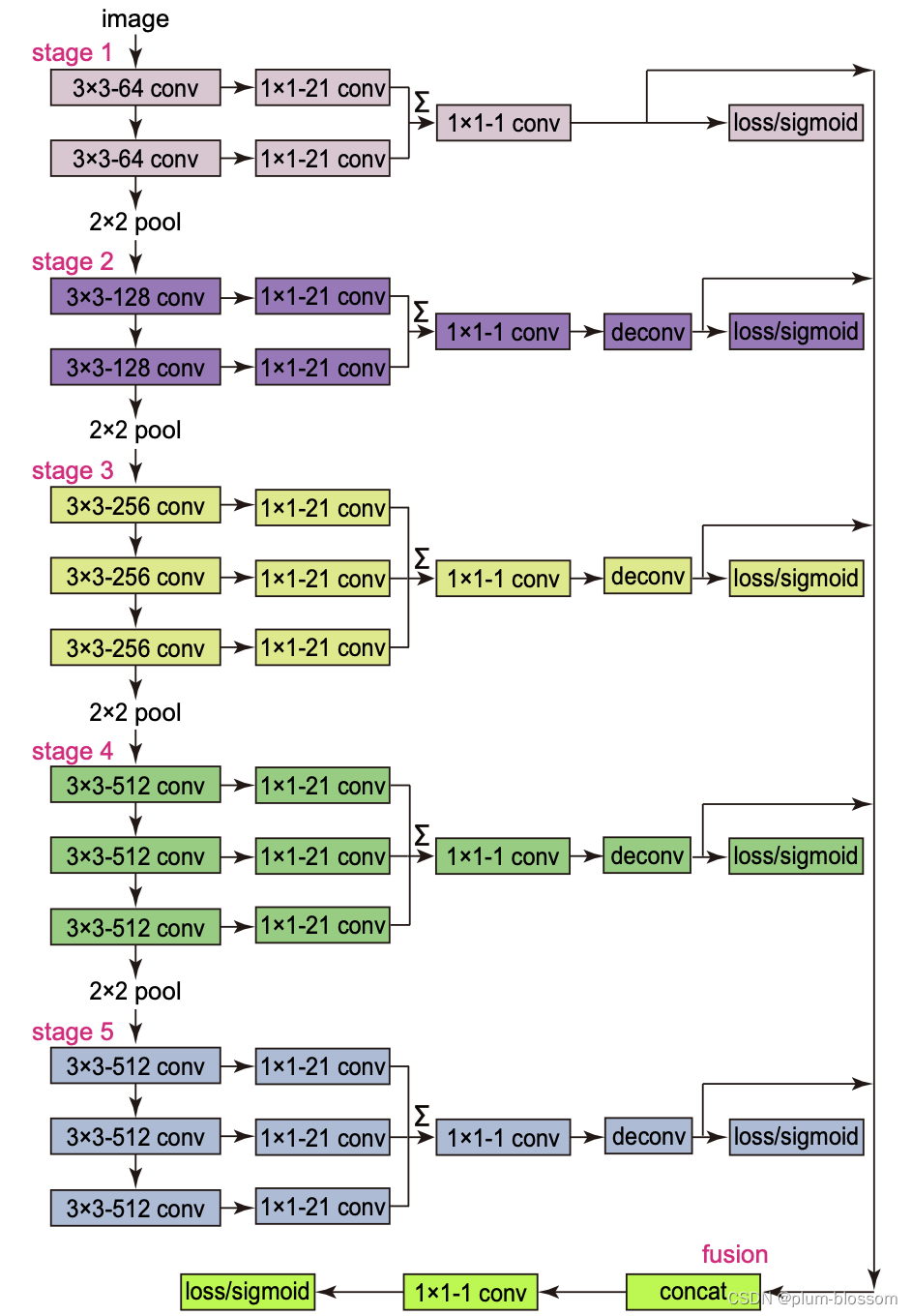
- VGG16中每个阶段中的每个卷积层都连接到核大小为1×1和通道深度为21的卷积层。每个阶段的特征映射都是用一个eltwise层(相加)来积累的,以获得混合特征。
- 一个1×1个卷积层跟随每个eltwise层。然后,使用一个反卷积层对这个特征映射进行上采样。
- 在每个阶段,交叉熵损失/Sigmoid连接到上采样层。
- 所有上采样层都是级联的。 然后使用1×1卷积从每个阶段融合特征映射。 最后,采用交叉熵损失/Sigmoid得到融合损失/输出
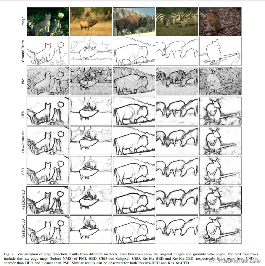
- RCF提供了一种比现有机制更好的机制来学习来自各级卷积特征的多尺度信息,作者认为这些特征都与边缘检测有关
- 在RCF中,高级特征较粗,可以在较大的对象或对象部分边界处获得强响应。
- 相比HED,RCF一是捕捉了所有conv的特征进行融合得到最终的结果,二是提出新的损失函数,三是提出多尺度测试
。
5.Crisp Edge Detection(CED)模型是前面介绍过的 HED 模型的另一种改进模型
CED 模型总体基于 HED 模型改造而来,其中做了如下几个改进:
-
将模型中的上采样操作从转置卷积插值更换为 PixelShuffle
-
添加了反向细化路径,即一个反向的从高层级特征逐步往低层级特征的边缘细化路径
-
没有多层级输出,最终的输出为融合了各层级的特征的边缘检测结果
架构图如下:

总结
本次实验主要对感受野、变种卷积、步长和零填充做了复习,实现二维卷积,利用自定义的二维卷积算子完成了一个简单的图片边缘检测,并且阅读了几篇边缘检测的论文。


 2970
2970


 被折叠的 条评论
为什么被折叠?
被折叠的 条评论
为什么被折叠?
 到【灌水乐园】发言


