


一种差分神经网络提高模型预测精度的方法
- 差分神经网络的提出
- 差分神经网络的实现
- 经过了不断的思考,得出了以下的方法
- 首先,先建立一个简单的神经网络,并选择 x = 0 → 10 x=0 \to 10 x=0→10 , y = s i n ( x ) y=sin(x) y=sin(x) 并进行标准化处理。
- S t e p 1 Step 1 Step1 进行简单拟合
- S t e p 2 Step 2 Step2 观察 y _ p r e 1 y\_pre1 y_pre1 和 y y y 之间的关系
- S t e p 3 Step 3 Step3 拟合 y _ p r e 1 y\_pre1 y_pre1 和 y y y 之间的关系
- S t e p 4 Step 4 Step4 拟合 1 − y _ p r e 1 1-y\_pre1 1−y_pre1 和 1 − y 1-y 1−y 之间的关系
- S t e p 5 Step 5 Step5 通过 y _ p r e 2 y\_pre2 y_pre2 与 y _ p r e 3 f y\_pre3f y_pre3f 求解 目前最终的 y _ p r e y\_pre y_pre
- 结果对比
- 直接预测
- 初始拟合图像
- 最终得分
- 优化后拟合图像
- 将整个过程进行封装后得到最终的差分神经网络模型,整个预测过程的优化使用同一神经网络模型(之后也可以根据需要使用异构的子神经网络),通过改进前后的结果对比,可以得出差分神经网络模型相比于传统神经网络模型有着更高的预测精度,降低了整体的系统误差。
- 在本次使用的案例中,预测数据的R2得分从0.985提升至0.993。但本次案例还有很多不足,由于时间原因还没有做测试数据集与预测数据集的划分,只是对比了简单的拟合效果,另外还没有做更多函数或者更多实际应用数据的测试。相信本次提出的差分神经网络模型能够有更好的表现,为实际应用带来更准确的学习与预测、为未来人工智能、大模型等领域通过跨学科的方法提供新的改进思路。
- 方向拓展
- 声明
差分神经网络的提出
最近再次受到模拟CMOS集成电路课程中差分放大器消除共模噪声的启发,想到将这种差分的思想运用到神经网络对预测的优化之中。
整个思考的过程还是遇到一些阻碍的,简单说就是放大器处理的是信号,进行简单的抽象就是对输入的有噪声的信号进行线性变化后进行输出,并在过程中消除了噪声的干扰。
输入往往可以看成
x
(
t
)
=
x
0
(
t
)
+
ϵ
(
t
)
x(t)=x_0(t)+\epsilon(t)
x(t)=x0(t)+ϵ(t) 而输出只是
y
(
t
)
=
A
x
(
t
)
y(t)=Ax(t)
y(t)=Ax(t)
因此可以通过两个将两组相位相反的信号
x
(
t
)
x(t)
x(t)与
−
x
(
t
)
-x(t)
−x(t)分别输入结构相同的放大电路得到
y
1
=
A
x
(
t
)
+
ϵ
(
t
)
y_1=Ax(t)+\epsilon(t)
y1=Ax(t)+ϵ(t)
y
2
=
−
A
x
(
t
)
+
ϵ
(
t
)
y_2=-Ax(t)+\epsilon(t)
y2=−Ax(t)+ϵ(t) ,然后通过
y
(
t
)
=
y
1
+
y
2
2
=
A
x
(
t
)
y(t)=\frac{y_1+y_2}{2}=Ax(t)
y(t)=2y1+y2=Ax(t) 可以消除系统带来的误差
而神经网络往往处理的是非线性的函数,是更复杂的映射关系。比如
x
x
x 为1到10,
y
=
s
i
n
(
x
)
y=sin(x)
y=sin(x) ,通过神经网络拟合后,假定为
y
′
=
s
i
n
(
x
)
+
ϵ
(
x
)
y'=sin(x)+\epsilon(x)
y′=sin(x)+ϵ(x),可以发现神经网络中
x
x
x 目前只是充当了放大器中的
t
t
t,训练好网络后即是输入
−
x
-x
−x 也不难预见网络也不会输出
−
s
i
n
(
x
)
-sin(x)
−sin(x) ,况且二者还有着不同的系统误差
ϵ
(
x
)
\epsilon(x)
ϵ(x) ,因此在这个过程中难以使用差分的思想。
差分神经网络的实现
经过了不断的思考,得出了以下的方法
首先,先建立一个简单的神经网络,并选择 x = 0 → 10 x=0 \to 10 x=0→10 , y = s i n ( x ) y=sin(x) y=sin(x) 并进行标准化处理。
import numpy as np
import matplotlib.pyplot as plt
from sklearn.metrics import r2_score

x = np.arange(0,10,0.1)

y = np.sin(x)

def preProcess(x):
    return (x - x.min()) / (x.max() - x.min())

x = preProcess(x)

y = preProcess(y)

x = x.reshape(len(x),1)

y = y.reshape(len(y),1)

def g(z,deriv=False):
    if deriv:
        return z*(1-z)
    return 1/(1+np.exp(-z))

def model1(x,theta1,theta2,theta3):
    z2 = np.dot(x,theta1)
    a2 = g(z2)
    z3 = np.dot(a2, theta2)
    a3 = g(z3)
    z4 = np.dot(a3, theta3)
    a4 = g(z4)
    return a2,a3,a4

def costFunc(h,y):
    j = (-1/len(y))*np.sum(y*np.log(h) + (1-y)*np.log(1-h))
    return j

def BP(a1,a2,a3,a4,theta1,theta2,theta3,alpha,y):
    # 求delta值
    delta4 = a4 - y
    delta3 = np.dot(delta4,theta3.T)*g(a3,True)
    delta2 = np.dot(delta3,theta2.T)*g(a2,True)

    # 求deltaTheta
    deltatheta3 = (1/len(y))*np.dot(a3.T,delta4)
    deltatheta2 = (1/len(y))*np.dot(a2.T,delta3)
    deltatheta1 = (1/len(y))*np.dot(a1.T,delta2)

    # 更新theta
    theta1 -= alpha*deltatheta1
    theta2 -= alpha*deltatheta2
    theta3 -= alpha*deltatheta3
    return theta1,theta2,theta3

len_a = 10
len_b = 10
def gradDesc(x,y,alpha=0.05,max_iter=500000,hidden_layer_size=(len_a,len_b)):
    m,n = x.shape
    k = y.shape[1]

    # 初始化theta
    theta1 = 2 * np.random.rand(n,hidden_layer_size[0]) - 1
    theta2 = 2 * np.random.rand(hidden_layer_size[0],hidden_layer_size[1]) - 1
    theta3 = 2 * np.random.rand(hidden_layer_size[1],k) - 1

    # 初始化代价
    j_history = np.zeros(max_iter)

    for i in range(max_iter):
        # 求预测值
        a2, a3, a4 = model1(x,theta1,theta2,theta3)
        # 记录代价
        j_history[i] = costFunc(a4,y)
        # 反向传播,更新参数
        theta1, theta2, theta3 = BP(x, a2, a3, a4, theta1, theta2, theta3, alpha, y)
        if i % 1000 == 0:
            print(i)
    return j_history,theta1, theta2, theta3
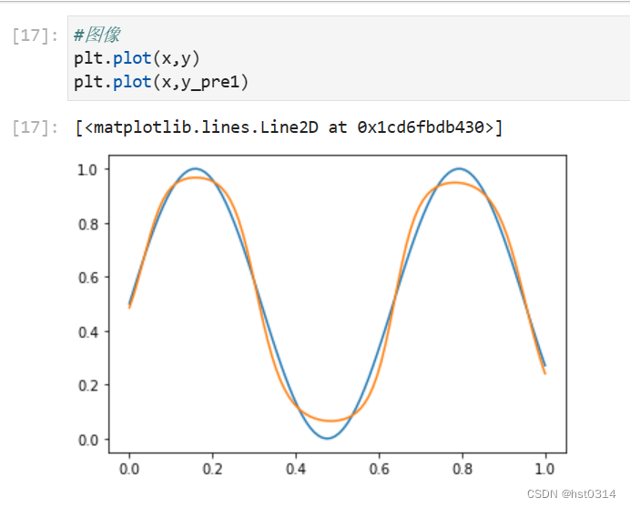
S t e p 1 Step 1 Step1 进行简单拟合
得到 x → y _ p r e 1 x \to y\_pre1 x→y_pre1的映射关系
j_history,theta1, theta2, theta3 = gradDesc(x,y)
a2, a3, y_pre1 = model1(x,theta1,theta2,theta3)

r2_score(y,y_pre1)  ##R2得分

#图像
plt.plot(x,y)
plt.plot(x,y_pre1)

S t e p 2 Step 2 Step2 观察 y _ p r e 1 y\_pre1 y_pre1 和 y y y 之间的关系
通过这一步确定出类似于信号的输入与输出,使其有更为接近线性的关系

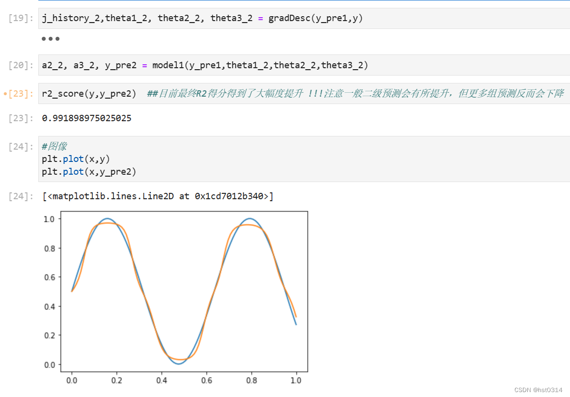
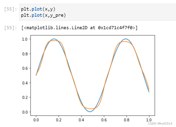
S t e p 3 Step 3 Step3 拟合 y _ p r e 1 y\_pre1 y_pre1 和 y y y 之间的关系
j_history_2,theta1_2, theta2_2, theta3_2 = gradDesc(y_pre1,y)
a2_2, a3_2, y_pre2 = model1(y_pre1,theta1_2,theta2_2,theta3_2)
r2_score(y,y_pre2)  ##目前最终R2得分得到了大幅度提升 !!!注意一般二级预测会有所提升,但更多组预测反而会下降
#图像
plt.plot(x,y)
plt.plot(x,y_pre2)
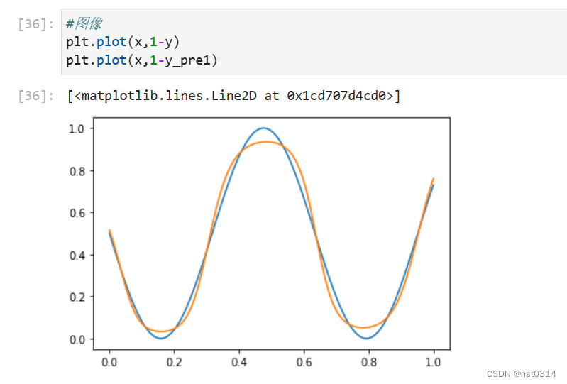
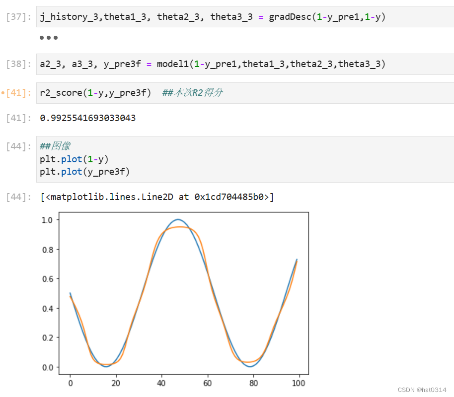
S t e p 4 Step 4 Step4 拟合 1 − y _ p r e 1 1-y\_pre1 1−y_pre1 和 1 − y 1-y 1−y 之间的关系
#图像
plt.plot(x,1-y)
plt.plot(x,1-y_pre1)
j_history_3,theta1_3, theta2_3, theta3_3 = gradDesc(1-y_pre1,1-y)
a2_3, a3_3, y_pre3f = model1(1-y_pre1,theta1_3,theta2_3,theta3_3)
r2_score(1-y,y_pre3f)  ##本次R2得分

##图像
plt.plot(1-y)
plt.plot(y_pre3f)
S t e p 5 Step 5 Step5 通过 y _ p r e 2 y\_pre2 y_pre2 与 y _ p r e 3 f y\_pre3f y_pre3f 求解 目前最终的 y _ p r e y\_pre y_pre
y_pre = (1+y_pre2-y_pre3f)/2

r2_score(y,y_pre) ##最终R2相比于最初得到了大幅度提高

plt.plot(y)
plt.plot(y_pre)

结果对比
直接预测

初始拟合图像
最终得分

优化后拟合图像


 9300
9300


 被折叠的 条评论
为什么被折叠?
被折叠的 条评论
为什么被折叠?
 到【灌水乐园】发言


