人工神经网络（ANN）：从背景到代码实现的详细解析

背景介绍

人工神经网络（Artificial Neural Network，ANN）是一种模拟人脑神经元网络结构和工作方式的计算模型，它由大量的神经元组成，并通过神经元之间的连接传递信息。ANN最早提出于上世纪50年代，但直到近年来，随着计算机技术和数据量的飞速发展，ANN才逐渐展现出强大的学习和处理能力，被广泛应用于机器学习和人工智能领域。

ANN的结构和原理

ANN由输入层、隐藏层和输出层组成，其中输入层接收外部输入数据，隐藏层对输入数据进行处理和转换，输出层产生最终的输出结果。每个神经元都有权重和偏置，权重用于调节输入信号的重要性，偏置用于调节神经元的激活程度。

ANN通过前向传播和反向传播两个过程来训练网络。前向传播时，输入数据经过权重和激活函数的处理，逐层传递至输出层，产生最终的输出结果；反向传播时，根据输出结果和真实标签之间的误差，通过梯度下降法更新权重和偏置，使网络逐渐收敛到最优状态。

代码分析

下面是一个简单的ANN实现，包括初始化、前向传播、反向传播和训练过程。我们以一个简单的示例来说明ANN的工作原理：

1. 初始化：初始化权重和偏置参数。
2. 前向传播：计算隐藏层和输出层的输出。
3. 反向传播：根据输出误差，更新权重和偏置。
4. 训练过程：迭代多次进行前向传播和反向传播，不断调整权重和偏置，直到网络收敛。

# 输入和输出数据
x = np.array([[0.05,0.1]])
y = np.array([[0.01,0.99]])

# 初始化神经网络
ann = ANN(input_shape=(1,2), hidden_shape1=(2,2), hidden_shape2=(2,2))

# 训练神经网络
ann.train(x, y, iterations=1000, learning_rate=0.05)

网络结构为：

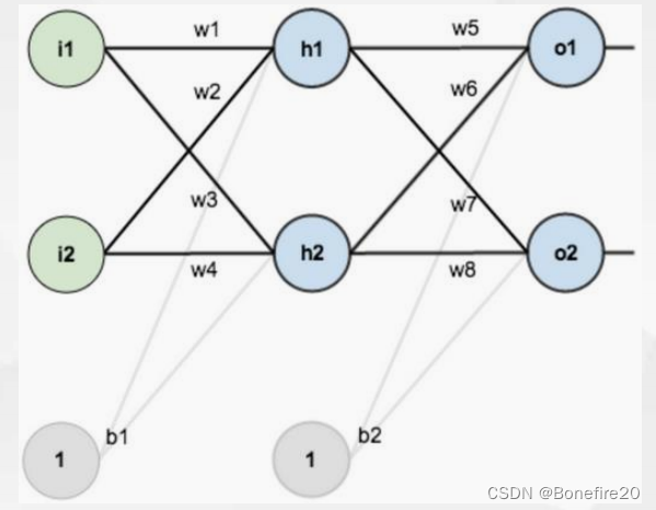
代码：

import numpy as np
import matplotlib.pyplot as plt

class ANN(object):
    def __init__(self,input_shape,hidden_shape1,hidden_shape2):
        self.input_shape = input_shape  #input_shape = 2
        self.hidden_shape = hidden_shape1 # hidden_shape1 = 2(input layer) x 2(hidden layer)
        self.output_shape = hidden_shape2 # hidden_shape2 = 2(hidden layer) x 2(output layer)
        self.initial()
        self.loss_history = []

    def initial(self):
        self.weight1 = np.random.uniform(-1,1,size=self.hidden_shape)
        # self.hidden_shape = (2,2) 第一个输入的形状2为输入层输入x的维度，第二个2表示隐藏层的数量
        self.b1 = np.random.uniform(-1,1,size=self.hidden_shape[1])
        self.weight2 = np.random.uniform(-1,1,size=self.output_shape)
        self.b2 = np.random.uniform(-1,1,size=self.output_shape[1])

    def sigmoid(self, x):
        return 1 / (1 + np.exp(-x))        

    def forward(self,x):

        self.hidden_layer = self.sigmoid(x@self.weight1+self.b1)
        self.output_layer = self.sigmoid(self.hidden_layer@self.weight2+self.b2)
        return self.output_layer
    
    def backward(self,output,x,learning_rate = 0.01):
        # Calculate the error for the output layer
        output_error = output - self.output_layer
        output_delta = output_error * self.output_layer * (1 - self.output_layer)
        
        # Calculate the error for the hidden layer
        hidden_error = output_delta @ self.weight2.T
        hidden_delta = hidden_error * self.hidden_layer * (1 - self.hidden_layer)
        
        # Update weights
        self.weight2 += learning_rate * self.hidden_layer.T @ output_delta
        self.b2 += learning_rate * output_delta.reshape(2)
        self.weight1 += learning_rate * x.T @ hidden_delta
        self.b1 += learning_rate * hidden_delta.reshape(2)

    def train(self,x,y,iterations = 100,learning_rate = 0.01):
        for i in range(iterations):
            output = self.forward(x)
            self.backward(y, x, learning_rate)
            
            # Calculate and store the loss
            loss = np.mean(np.square(y - output))
            self.loss_history.append(loss)
        
        # Print final predictions
        final_output = self.forward(x)
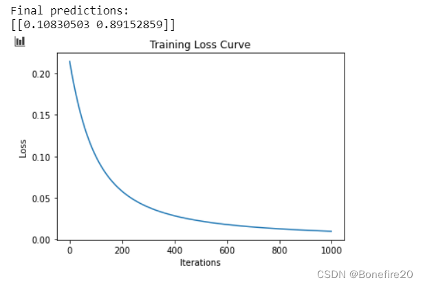
        print("Final predictions:")
        print(final_output)

        # Plot the loss curve
        plt.plot(range(iterations), self.loss_history)
        plt.xlabel('Iterations')
        plt.ylabel('Loss')
        plt.title('Training Loss Curve')
        plt.show()

# 输入和输出数据
x = np.array([[0.05,0.1]])
y = np.array([[0.01,0.99]])

# 初始化神经网络
ann = ANN(input_shape=(1,2), hidden_shape1=(2,2), hidden_shape2=(2,2))

# 训练神经网络
ann.train(x, y, iterations=1000, learning_rate=0.05)