


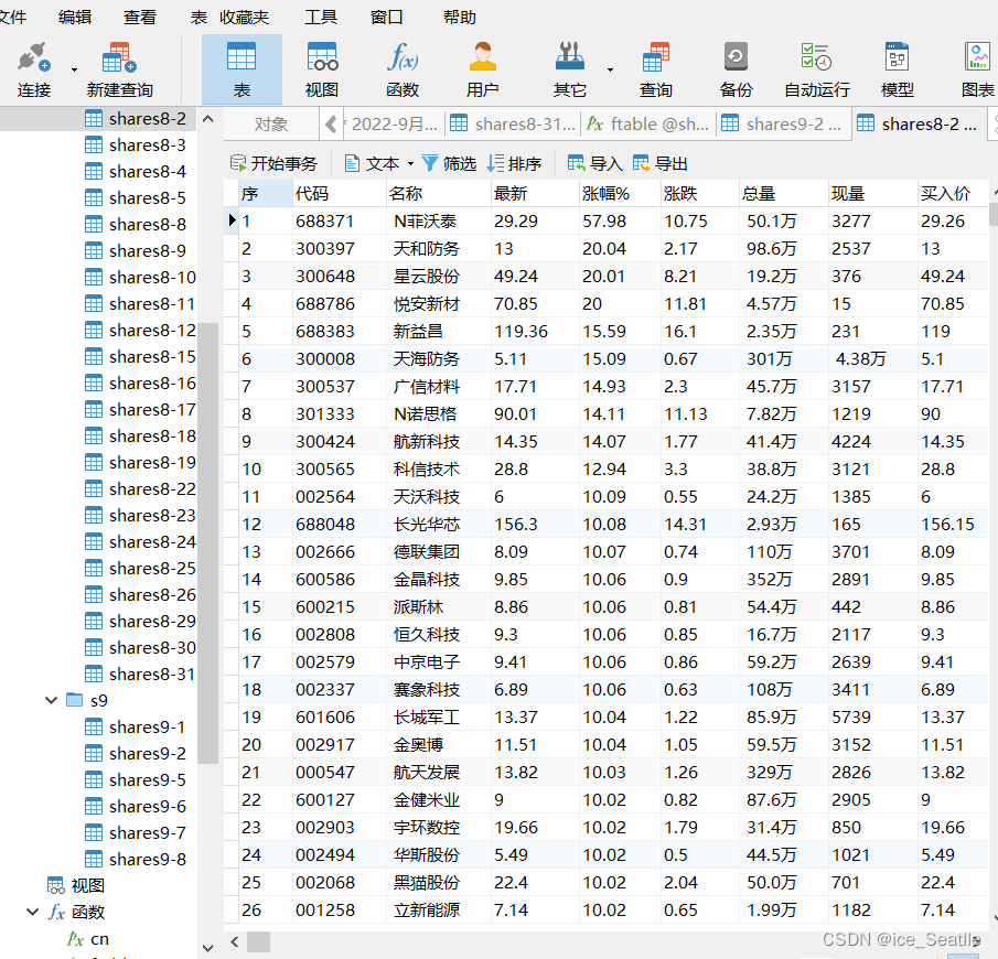
一.数据库导入股票数据
爬虫或其他工具获取数据,并转换为Excel表,然后导入数据库中.
我的如下:
二.创建函数,编写存储过程
1.mysql存储过程
CREATE DEFINER=`root`@`localhost` PROCEDURE `trendp`(in s_name varchar(20))
BEGIN
			declare i int default 0;
    while(i<1)do
		select
		a.`涨幅%`'8-2',
		b.`涨幅%`'8-3',
		c.`涨幅%`'8-4',
		d.`涨幅%`'8-5',
		e.`涨幅%`'8-8',
		f.`涨幅%`'8-9',
		DENSE_RANK()over(order by a.`代码` asc) from `shares8-2` a
		join `shares8-3` b on a.`代码`=b.`代码`
		join `shares8-4` c on b.`代码`=c.`代码`
		join `shares8-5` d on c.`代码`=d.`代码`
		join `shares8-8` e on  d.`代码`=e.`代码`
		join `shares8-9` f on e.`代码`=f.`代码`
		where a.`名称` like concat('%',s_name,'%');
        set i=i+1;
    end while;

END
其中以6日结果为例,进行连表并使用窗口函数over()拼接在一起,进行数据排序,以区分数据来源
2.Navicat中调用测试:
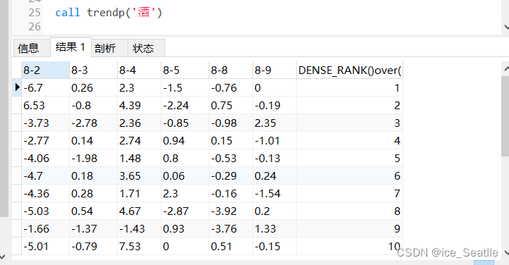
因为要对数据集进行处理,索引不查询股票代码和名称
三.编写python准备及思路
导入相关库,其中MySQLdb用来连接数据库并产生数据,使用pandas处理数据,使用xlwings处理excal表格,使用matplotlib进行对数据可视化操作,使用time计算程序运行时间
import MySQLdb
import pandas as pd
import matplotlib.pyplot as plt
import xlwings as xw
import time
由于各种数据传递相关联,先看总代码
四.完整代码:
# _*_ coding:utf-8 _*_
# @Time : 2022/9/8 13:26
# @Author : ice_Seattle
# @File : trend_point.py
# @Software: PyCharm
import MySQLdb
import pandas as pd
import matplotlib.pyplot as plt
import xlwings as xw
import time
t1 = time.time()
# 打开数据库连接
db = MySQLdb.connect("localhost", "root", "489000", "shares2022", charset='utf8')
# 使用cursor()方法获取操作游标
cursor = db.cursor()
# 使用execute方法执行SQL语句
cursor.execute("SELECT VERSION()")
# 使用 fetchone() 方法获取一条数据
version = cursor.fetchone()
print("Database version : %s " % version)
name = '埃斯顿'
sql = f"""CALL trendp('{name}') """
cursor.execute(sql)
# 定义列表, 循环下标
list1 = []
for i in range(1, 10000):
data = cursor.fetchone()
if data is None:
break
else:
for j in range(1, 7):
list1.append(data[j-1])
r = list1
# 关闭数据库连接
db.close()
x = ['8-2', '8-3', '8-4', '8-5', '8-8', '8-9']
y = [r[0], r[1], r[2], r[3], r[4], r[5]]
df1 = pd.DataFrame({
x[0]: y[0],
x[1]: y[1],
x[2]: y[2],
x[3]: y[3],
x[4]: y[4],
x[5]: y[5]
}, index=[0])
path = 'E:/py/trend_point.xlsx'
df1.to_excel(path, sheet_name='Sheet1', index=False)
app = xw.App(visible=True, add_book=False)
app.display_alerts = False
app.screen_updating = True
wb = app.books.open(path)
sht = wb.sheets.active # 获取当前活动的工作表
titles = sht.range('A1:F1')
titles.api.HorizontalAlignment = -4108 # 水平居中
sht.range('A1:F1').color = (217, 217, 217)
A1 = sht['A1:F2']
"""设置边框"""
# Borders(11) 内部垂直边线。
A1.api.Borders(11).LineStyle = 1
A1.api.Borders(11).Weight = 2
#
# Borders(12) 内部水平边线。
A1.api.Borders(12).LineStyle = 1
A1.api.Borders(12).Weight = 2
# LineStyle = 1 直线。
A1.api.Borders(9).LineStyle = 1
A1.api.Borders(9).Weight = 2 # 设置边框粗细。
A1.api.Borders(10).LineStyle = 1
A1.api.Borders(10).Weight = 2
A1.api.HorizontalAlignment = -4108 # 水平居中
A1.api.VerticalAlignment = -4130 # 自动换行对齐
df = pd.read_excel(path, index_col=None)
print(df)
a = x
b = df.iloc[0].tolist()
print("最终涨幅百分比", round(df.iloc[0].sum(), 2))
# 调用绘制方法
plt.rcParams['font.sans-serif'] = ['SimHei'] # 用来正常显示中文标签
plt.rcParams['axes.unicode_minus'] = False # 用来正常显示负号
# 给图标添加标题
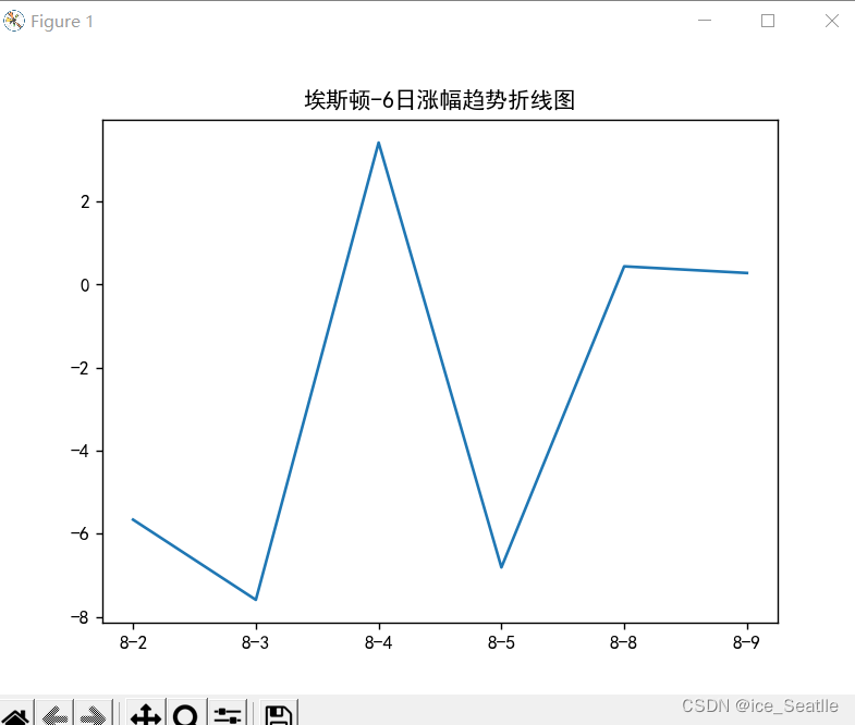
plt.title(f'{name}-6日涨幅趋势折线图')
plt.plot(a, b)
# 保存图
plt.savefig(f'{name}-6日趋势.png')
# 用时计算
t2 = time.time()
t = t2-t1
t = round(t, 2)
print('用时'+str(t)+'秒')
print('done!!')
# 显示图
plt.show()
wb.save(r'./trend_point.xlsx')
app.quit()
五.运行结果
1.python终端区
Database version : 8.0.29
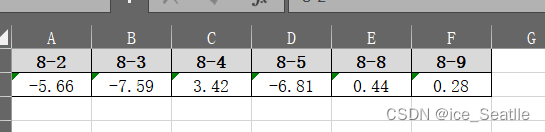
8-2 8-3 8-4 8-5 8-8 8-9
0 -5.66 -7.59 3.42 -6.81 0.44 0.28
最终涨幅百分比 -15.92
用时2.29秒
done!!
2.简易折线图
3.excel数据
每次的图片都会保存在本地,只需要在name中赋给不同的值,因为存储过程使用的模糊查询,索引部分股票可以简写,对于批量生成暂且不涉及
六.分部流程讲解
1.数据库部分
t1 = time.time()
# 打开数据库连接
db = MySQLdb.connect("localhost", "root", "489000", "shares2022", charset='utf8')
# 使用cursor()方法获取操作游标
cursor = db.cursor()
# 使用execute方法执行SQL语句
cursor.execute("SELECT VERSION()")
# 使用 fetchone() 方法获取一条数据
version = cursor.fetchone()
print("Database version : %s " % version)
name = '埃斯顿'
sql = f"""CALL trendp('{name}') """
cursor.execute(sql)
# 定义列表, 循环下标
list1 = []
for i in range(1, 10000):
    data = cursor.fetchone()
    if data is None:
        break
    else:
        for j in range(1, 7):
            list1.append(data[j-1])
r = list1
# 关闭数据库连接
db.close()
t1用来记录起始运行时刻,使用MySQLdb库相关方法进行获取数据库中的值,
其中sql中CALL trendp()为调用数据库中的存储过程此处以name赋值,f'{name}格式进行输出
然后循环游标读取数据库中数据,如果数据为空,则终止读取,不为空就输出,并将数据循环输入到定义的列表中,因为只需要6日数据点,所以在此range(1,7)
2.pandas处理
x = ['8-2', '8-3', '8-4', '8-5', '8-8', '8-9']
y = [r[0], r[1], r[2], r[3], r[4], r[5]]
df1 = pd.DataFrame({
    x[0]: y[0],
    x[1]: y[1],
    x[2]: y[2],
    x[3]: y[3],
    x[4]: y[4],
    x[5]: y[5]
}, index=[0])
path = 'E:/py/trend_point.xlsx'
df1.to_excel(path, sheet_name='Sheet1', index=False)
其中x为日期,y为数据库中每一个对应日期的数据,因为为列表,所以可以调用列表下标,此时数据形参二维,笛卡尔坐标系
将数据以字典样式关联起来并转换为DataFrame的格式
其中设置行索引的值为0,即index=[0],注意,此索引中设置不能为非数字,否则报错
定义路径path,此处为我的绝对路径
使用df1.to_excel()将数据写入到excel表中
3.对excal中标准化
app = xw.App(visible=True, add_book=False)
app.display_alerts = False
app.screen_updating = True
wb = app.books.open(path)
sht = wb.sheets.active  # 获取当前活动的工作表
titles = sht.range('A1:F1')
titles.api.HorizontalAlignment = -4108   # 水平居中
sht.range('A1:F1').color = (217, 217, 217)
A1 = sht['A1:F2']
"""设置边框"""
# Borders(11) 内部垂直边线。
A1.api.Borders(11).LineStyle = 1
A1.api.Borders(11).Weight = 2
#
# Borders(12) 内部水平边线。
A1.api.Borders(12).LineStyle = 1
A1.api.Borders(12).Weight = 2

# LineStyle = 1 直线。
A1.api.Borders(9).LineStyle = 1
A1.api.Borders(9).Weight = 2               # 设置边框粗细。
A1.api.Borders(10).LineStyle = 1
A1.api.Borders(10).Weight = 2
A1.api.HorizontalAlignment = -4108   # 水平居中
A1.api.VerticalAlignment = -4130    # 自动换行对齐
这里主要为设置样式,xw.App中visible属性为设置是否可见excel,True会在后台打开
其中设置了A1:F1的标题格式,并设置了此区间的颜色rbg(217,217,217),并将A1范围内进行边框设置
4.数据可视化,生成6日图
df = pd.read_excel(path, index_col=None)
print(df)
a = x
b = df.iloc[0].tolist()
print("最终涨幅百分比", round(df.iloc[0].sum(), 2))
# 调用绘制方法
plt.rcParams['font.sans-serif'] = ['SimHei']  # 用来正常显示中文标签
plt.rcParams['axes.unicode_minus'] = False   # 用来正常显示负号
# 给图标添加标题
plt.title(f'{name}-6日涨幅趋势折线图')
plt.plot(a, b)
# 保存图
plt.savefig(f'{name}-6日趋势.png')
# 用时计算
t2 = time.time()
t = t2-t1
t = round(t, 2)
print('用时'+str(t)+'秒')
print('done!!')
# 显示图
plt.show()
wb.save(r'./trend_point.xlsx')
app.quit()
df为读取excal中的数据,path为上面设置过的绝对路径
设置a,b两个参数,目的是横纵坐标显示,其中df.iloc[0]为查询之前设置行索引index[0]那一行的数据,然后使用tolist转换为列表形式
使用plt.savefig保存图片,计算程序运行到此处t的时间
最后使用plt.show显示图片
至此,操作完成,再也不需要频繁调用存储过程查看了
END


 被折叠的 条评论
为什么被折叠?
被折叠的 条评论
为什么被折叠?
 到【灌水乐园】发言


