【Intel校企合作课程】预测淡水质量

一、问题描述

         淡水是我们最重要和最稀缺的自然资源之一，仅占地球总水量的 3%。它几乎触及我们日常生活的方方面面，从饮用、游泳和沐浴到生产食物、电力和我们每天使用的产品。获得安全卫生的供水不仅对人类生活至关重要，而且对正在遭受干旱、污染和气温升高影响的周边生态系统的生存也至关重要。

        预测淡水是否可以安全饮用和被依赖淡水的生态系统所使用，从而可以帮助全球水安全和环境可持续性发展。

二、数据集

2.1 数据集描述

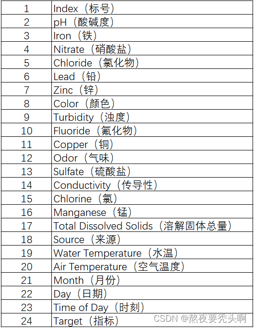
        该数据集包含了淡水的特征元素和标签。共有24列，具体特征含义如下图所示。

2.2 数据集下载

        训练集下载地址：https://filerepo.idzcn.com/hack2023/datasetab75fb3.zip

        测试集下载地址：百度网盘 请输入提取码

三、工具集

        使用英特尔oneAPI Developer Cloud，借助云平台提供的计算节点等硬件资源完成，并使用 英特尔® ONEAPI AI分析工具包。

四、代码

4.1 上传数据集

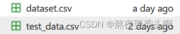
        通过上方链接下载数据集后，可在本地解压，然后再上传至云平台。

 4.2 加载第三方库

import modin.pandas as pd
import os
os.environ["MODIN_ENGINE"] = "dask"
from modin.config import Engine
Engine.put("dask")

 4.3 查看数据集

import pandas
data = pandas.read_csv('dataset.csv')
print('数据规模：{}\n'.format(data.shape))
display(data.head())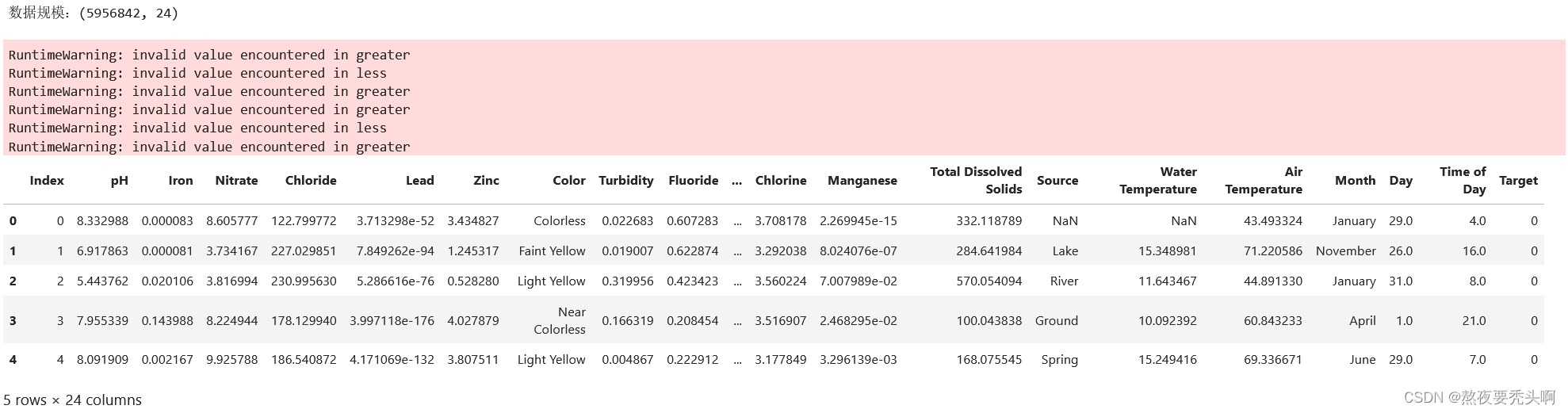

print(data.describe())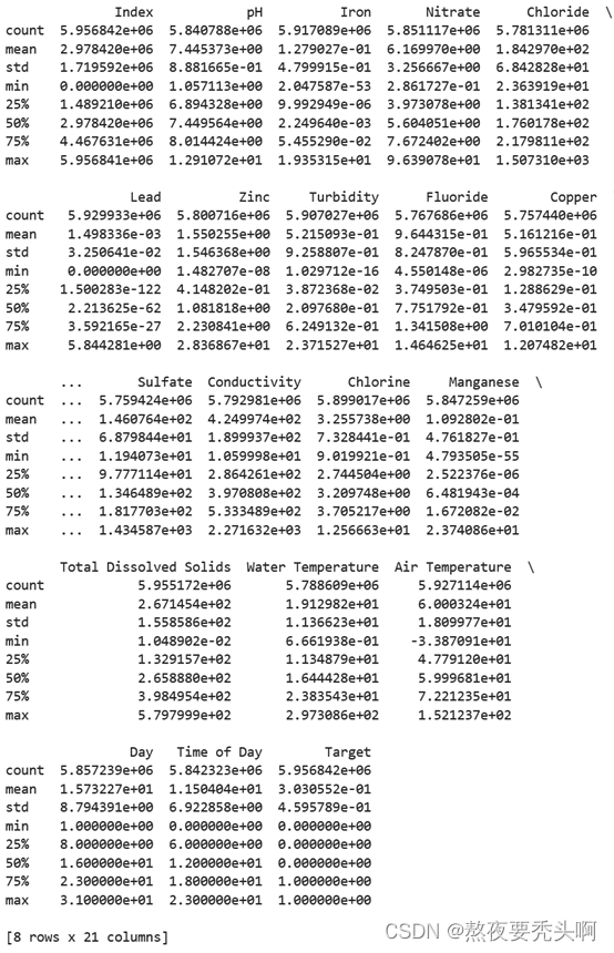

data=data.infer_objects()
data.info()

4.4 数据可视化

import matplotlib.pyplot as plt
 
def plot_target(target_col):
    tmp=data[target_col].value_counts(normalize=True)
    target = tmp.rename(index={1:'Target 1',0:'Target 0'})
    wedgeprops = {'width':0.8, 'linewidth':10}
    
    plt.figure(figsize=(8,8))
    plt.pie(list(tmp), labels=target.index,
            startangle=90, autopct='%1.2f%%',wedgeprops=wedgeprops)
    plt.title('Label Distribution', fontsize=16)
    plt.show() 
    
plot_target(target_col='Target')

饼状图

import seaborn as sns
 
figData=data.drop(columns=['Index','Source','Color','Month','Target'])
sns.set_style('ticks')      # 设置了seaborn的绘图风格为'ticks'，更改轴线样式
# 设置了seaborn的上下文为'notebook'，并调整了字体大小
sns.set_context('notebook', font_scale=1.1)
# column = data.drop(columns=['Index','Source','Color','Month','Target']).columns.tolist()
# 从data数据框中移除了不需要的列，并将剩下的列转化为列表格式并存储在column变量中
plt.figure(figsize=(30, 15))        # 创建一个新的图形，大小为20x10英寸
for i,column in enumerate(figData.columns,start=1):     # 循环显示箱线图
    plt.subplot(5,4,i)
    sns.boxplot(y=column, data=figData, width=0.6)
    plt.ylabel(column, fontsize=12)
plt.tight_layout()      # 优化图形布局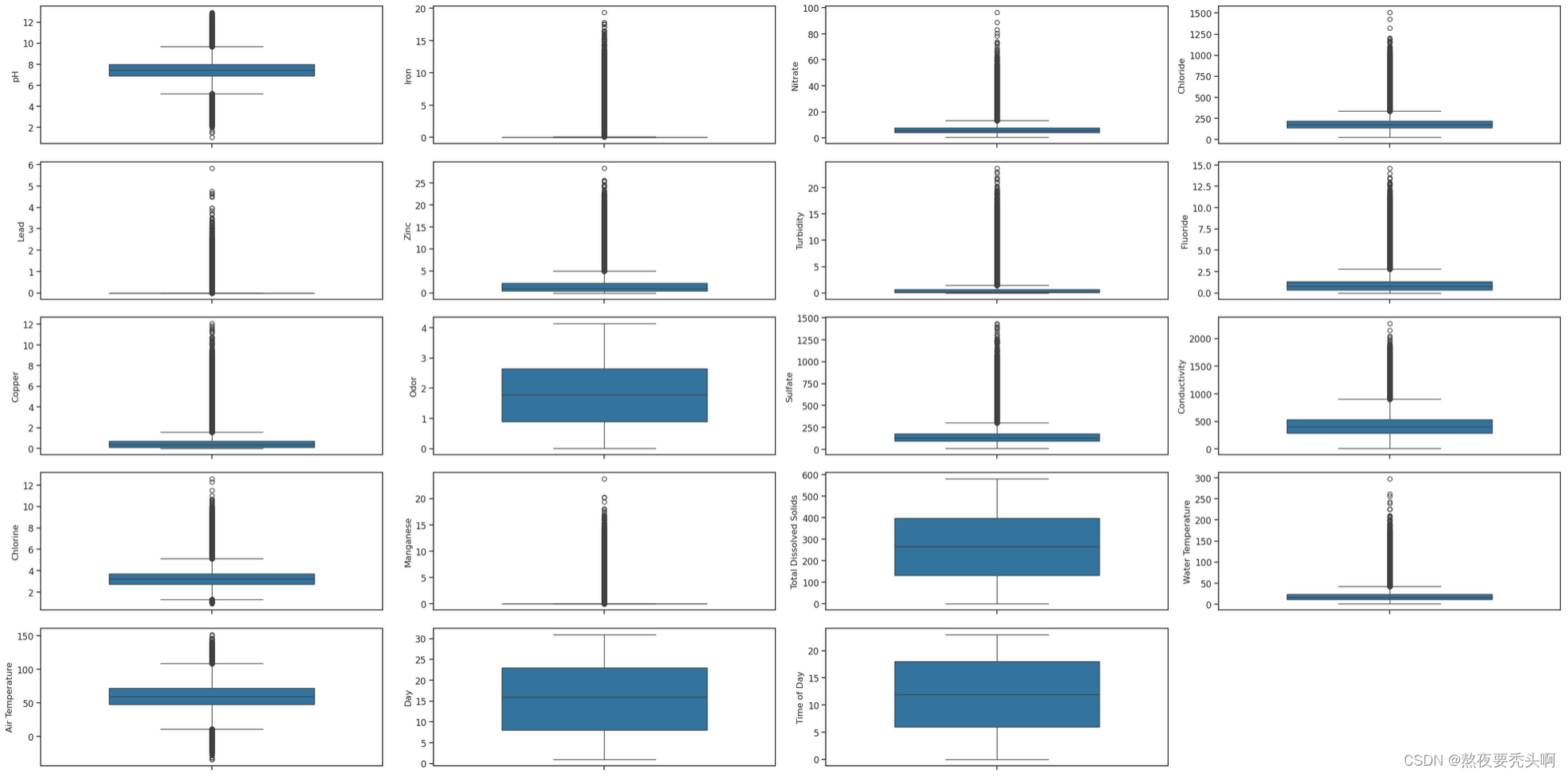

箱型图

 4.5 数据预处理

数据预处理可以确保数据的准确性和完整性，避免一些错误数据对结果准确性的影响。

4.5.1 查看缺失值和重复值

check_data=data.drop(columns=['Index'])    # 去除Index(标号)
missing = check_data.isna().sum().sum()    # 缺失值统计
duplicates = check_data.duplicated().sum() # 重复值统计
print("\n数据集中有{:,.0f} 缺失值.".format(missing))
print("数据集中有 {:,.0f} 重复值.".format(duplicates))

4.5.2 处理缺失值和重复值

        从上述结果可以看出，数据集中的缺失值和重复值太多，不能够采用直接删除的方法。观察数据集，可以发现其中有三列的数据为字符类型，非线性数据，对于这三列中的缺失值可以采用直接删除的方法；其余列的数据都是线性的数值类数据，采用线性插值来进行填充。

columns_check=['Source','Color','Month']    # 去除字符列中缺失值
data_target_na = check_data[check_data['Target'].isna()]
na_index = list(data_target_na.index)
check_data = check_data.drop(na_index)
check_data=check_data.dropna(subset=columns_check)
check_data=check_data.fillna(check_data.interpolate())   # 其余部分线性填充
check_data.drop_duplicates(keep='first', inplace=True, ignore_index=True)
 
missing = check_data.isna().sum().sum()
duplicates = check_data.duplicated().sum()
print("\n数据集中有{:,.0f} 缺失值.".format(missing))
print("数据集中有 {:,.0f} 重复值.".format(duplicates))

 4.5.3 平衡数据

from imblearn.over_sampling import SMOTE
new_data = check_data.drop(columns=columns_check) # 经过数据处理后的数据
smote_model = SMOTE(k_neighbors=2,random_state=123,sampling_strategy=1/2)
x_smote,y_smote = smote_model.fit_resample(new_data.drop(columns=['Target']),new_data['Target'])
df_smote = pd.concat([x_smote, y_smote], axis=1)
df_smote.groupby('Target').count()

 4.5.4 过拟合与欠拟合

from imblearn.over_sampling import RandomOverSampler
from imblearn.under_sampling import RandomUnderSampler
rus = RandomUnderSampler(random_state=0,sampling_strategy=1/2)
ros = RandomOverSampler(random_state=0,sampling_strategy=1/2)
X_resampled, y_resampled = ros.fit_resample(new_data.drop(columns=['Target']),new_data['Target'])
df_resampled = pd.concat([X_resampled, y_resampled], axis=1)
X_uresampled, y_uresampled = rus.fit_resample(new_data.drop(columns=['Target']),new_data['Target'])
df_uresampled = pd.concat([X_uresampled, y_uresampled], axis=1)
df_new = pd.concat([df_smote, df_resampled[df_resampled['Target']==1.0]], axis=0)
df_new = pd.concat([df_new[df_new['Target']==1.0],df_uresampled[df_uresampled['Target']==0.0]])
df_new.groupby('Target').count()

 4.6 定义函数

        prepare_train_test_data()为准备训练集和对应验证集，plot_model_res()为绘制模型效果图像函数，plot_distribution()为分布图像函数，用于将训练过程效果可视化。

import plotly.io as pio
pio.renderers.default = "iframe"
def prepare_train_test_data(data, target_col, test_size):
    
    scaler = RobustScaler()   
    X = data.drop(target_col, axis=1)
    y = data[target_col]
    X_train, X_test, y_train, y_test = train_test_split(X, y, test_size=test_size, random_state=21)
    X_train_scaled = scaler.fit_transform(X_train)
    X_test_scaled = scaler.transform(X_test)
    print("Train Shape: {}".format(X_train_scaled.shape))
    print("Test Shape: {}".format(X_test_scaled.shape))
    
    return X_train_scaled, X_test_scaled, y_train, y_test
 
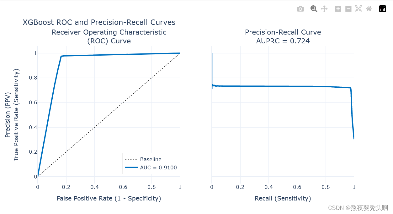
def plot_model_res(model_name, y_test, y_prob):
    
    intel_pal=['#0071C5','#FCBB13']
    color=['#7AB5E1','#FCE7B2']
    
    fpr, tpr, _ = roc_curve(y_test, y_prob)
    roc_auc = auc(fpr,tpr)
    precision, recall, _ = precision_recall_curve(y_test, y_prob)
    auprc = average_precision_score(y_test, y_prob)
    
    fig = make_subplots(rows=1, cols=2, 
                        shared_yaxes=True, 
                        subplot_titles=['Receiver Operating Characteristic<br>(ROC) Curve',
                                        'Precision-Recall Curve<br>AUPRC = {:.3f}'.format(auprc)])
    
    fig.add_trace(go.Scatter(x=np.linspace(0,1,11), y=np.linspace(0,1,11), 
                             name='Baseline',mode='lines',legendgroup=1,
                             line=dict(color="Black", width=1, dash="dot")), row=1,col=1)    
    fig.add_trace(go.Scatter(x=fpr, y=tpr, line=dict(color=intel_pal[0], width=3), 
                             hovertemplate = 'True positive rate = %{y:.3f}, False positive rate = %{x:.3f}',
                             name='AUC = {:.4f}'.format(roc_auc),legendgroup=1), row=1,col=1)
    fig.add_trace(go.Scatter(x=recall, y=precision, line=dict(color=intel_pal[0], width=3), 
                             hovertemplate = 'Precision = %{y:.3f}, Recall = %{x:.3f}',
                             name='AUPRC = {:.4f}'.format(auprc),showlegend=False), row=1,col=2)
    fig.update_layout(template=temp, title="{} ROC and Precision-Recall Curves".format(model_name), 
                      hovermode="x unified", width=900,height=500,
                      xaxis1_title='False Positive Rate (1 - Specificity)',
                      yaxis1_title='True Positive Rate (Sensitivity)',
                      xaxis2_title='Recall (Sensitivity)',yaxis2_title='Precision (PPV)',
                      legend=dict(orientation='v', y=.07, x=.45, xanchor="right",
                                  bordercolor="black", borderwidth=.5))
    fig.show()
 
def plot_distribution(y_prob): 
    plot_df=pd.DataFrame.from_dict({'Target 0':(len(y_prob[y_prob<=0.5])/len(y_prob))*100, 
                                    'Target 1':(len(y_prob[y_prob>0.5])/len(y_prob))*100}, 
                                   orient='index', columns=['pct'])
    fig=go.Figure()
    fig.add_trace(go.Pie(labels=plot_df.index, values=plot_df.pct, hole=.45, 
                         text=plot_df.index, sort=False, showlegend=False,
                         marker=dict(colors=color,line=dict(color=intel_pal,width=2.5)),
                         hovertemplate = "%{label}: <b>%{value:.2f}%</b><extra></extra>"))
    fig.update_layout(template=temp, title='Predicted Target Distribution',width=700,height=450,
                      uniformtext_minsize=15, uniformtext_mode='hide')
    fig.show()

 4.7 训练模型

        使用XGBoost模型来解决二分类问题，并使用Intel 的 Data Analytics Acceleration Library (DAAL) 的 Python 接口来进行优化加速。结果以F1分数和ROC 曲线下面积 (AUC)作为评价标准。

from sklearnex import patch_sklearn
import daal4py as d4p
patch_sklearn()
from sklearn.model_selection import train_test_split, StratifiedKFold, GridSearchCV, RandomizedSearchCV
from sklearn.preprocessing import RobustScaler
from sklearn.metrics import roc_auc_score, roc_curve, auc, accuracy_score, f1_score
from sklearn.metrics import precision_recall_curve, average_precision_score
from xgboost.sklearn import XGBClassifier
import warnings
import numpy as np
import plotly.graph_objects as go  
from plotly.subplots import make_subplots
warnings.filterwarnings("ignore")
 
import time
import warnings
 
## Prepare Train and Test datasets ##
print("Preparing Train and Test datasets")
X_train, X_test, y_train, y_test = prepare_train_test_data(data=new_data,
                                                            target_col='Target', 
                                                            test_size=0.2)
    
## Initialize XGBoost model ##
ratio = float(np.sum(y_train == 0)) / np.sum(y_train == 1)
parameters = {'scale_pos_weight': ratio.round(2), 
                'tree_method': 'hist',
                'random_state': 21}
xgb_model = XGBClassifier(**parameters)
 
## Tune hyperparameters ##
strat_kfold = StratifiedKFold(n_splits=3, shuffle=True, random_state=21)
print("\nTuning hyperparameters..")
grid = {'min_child_weight': [1, 5, 10, 15],
        'gamma': [0.5, 1, 1.5, 2, 5],
        'max_depth': [3, 4, 5, 6],
        }
 
grid_search = GridSearchCV(xgb_model, param_grid=grid, 
                            cv=strat_kfold, scoring='roc_auc', 
                            verbose=1, n_jobs=-1)
start = time.time()
grid_search.fit(X_train, y_train)
end = time.time()
 
print("Done!\nBest hyperparameters:", grid_search.best_params_)
print("Best cross-validation AUC: {:.4f}".format(grid_search.best_score_))
    
## Convert XGB model to daal4py ##
xgb = grid_search.best_estimator_
 
daal_model = d4p.get_gbt_model_from_xgboost(xgb.get_booster())
 
## Calculate predictions ##
daal_prob = d4p.gbt_classification_prediction(nClasses=2,
    resultsToEvaluate="computeClassLabels|computeClassProbabilities",
    fptype='float').compute(X_test, daal_model).probabilities # or .predictions
xgb_pred = pd.Series(np.where(daal_prob[:,1]> 0.5, 1, 0), name='Target')
xgb_auc = roc_auc_score(y_test, daal_prob[:,1])
xgb_f1 = f1_score(y_test, xgb_pred)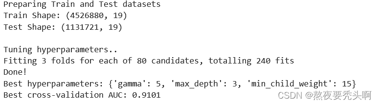

 4.8 保存模型

xgb.save_model('xgb_model.model')

4.9 训练结果可视化

temp = 'plotly_white'
intel_pal=['#0071C5','#FCBB13']
color=['#7AB5E1','#FCE7B2']
print('模型拟合时间:{:.2f}'.format(end-start))
print("\nTest F1 Accuracy: {:.2f}%, AUC: {:.5f}".format(xgb_f1*100, xgb_auc)) 
plot_model_res(model_name='XGBoost', y_test=y_test, y_prob=daal_prob[:,1])

plot_distribution(daal_prob[:,1])
print('预测类别为0的数量为:{:d}'.format(len(daal_prob[:,1][daal_prob[:,1]<=0.5])))
print('预测类别为1的数量为:{:d}'.format(len(daal_prob[:,1][daal_prob[:,1]>=0.5])))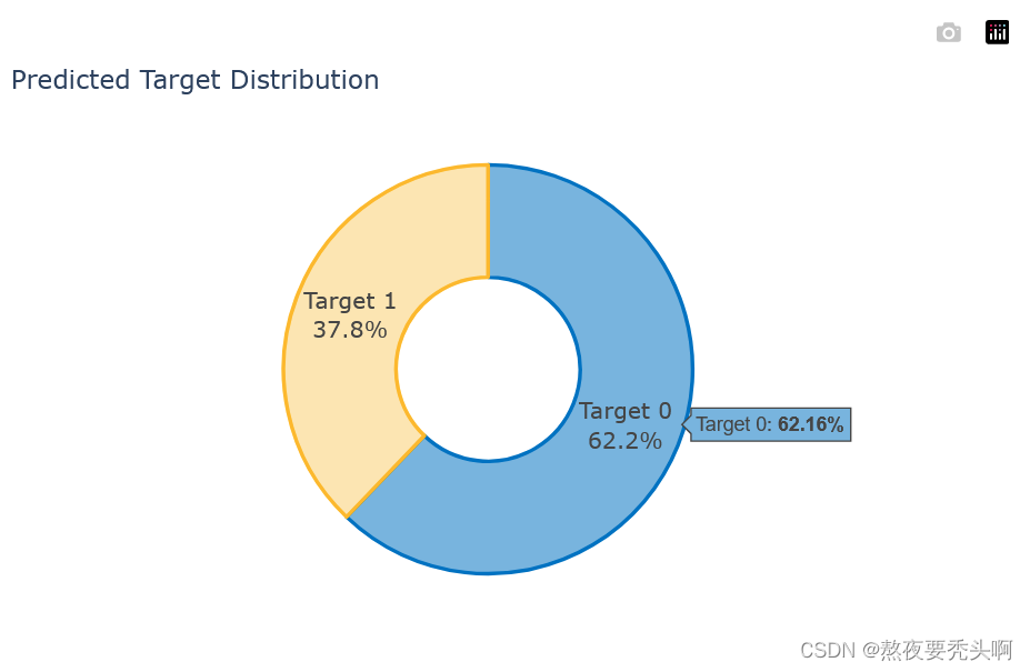

4.10 测试集预测推理

 4.10.1 读取测试集

test = pandas.read_csv('test_data.csv')
columns_check = columns_check=['Index','Source','Color','Month'] 

4.10.2 预测推理并打印结果

from sklearn.metrics import roc_auc_score, roc_curve, auc, accuracy_score, f1_score
import xgboost as xgb
from sklearnex import patch_sklearn
import daal4py as d4p
patch_sklearn()
from sklearn.model_selection import train_test_split, StratifiedKFold, GridSearchCV, RandomizedSearchCV
from sklearn.preprocessing import RobustScaler
from sklearn.metrics import roc_auc_score, roc_curve, auc, accuracy_score, f1_score
from sklearn.metrics import precision_recall_curve, average_precision_score
from xgboost.sklearn import XGBClassifier
import warnings
import numpy as np
import plotly.graph_objects as go  
from plotly.subplots import make_subplots
warnings.filterwarnings("ignore")
 
import time
import warnings
Y_true = test['Target']
new_test = test.drop(columns=columns_check)
new_test = new_test.drop(columns='Target')

scaler = RobustScaler()
X_test = scaler.fit_transform(new_test)
model_file = './xgb_model.model'
start = time.time()
xgb_model = xgb.Booster()
xgb_model.load_model(model_file)
 
daal_model = d4p.get_gbt_model_from_xgboost(xgb_model)
#daal_model = d4p.get_gbt_model_from_xgboost(xgb_model.get_booster()) 

## Calculate predictions ##
 
daal_prob = d4p.gbt_classification_prediction(nClasses=2,
                                              resultsToEvaluate="computeClassLabels|computeClassProbabilities",
                                              fptype='float').compute(X_test, daal_model).probabilities   # probabilities # or .predictions

end = time.time()

xgb_pred = pd.Series(np.where(daal_prob[:,1]>.5, 1, 0), name='Target')
f1 = f1_score(Y_true, xgb_pred) 
print('推理时间:{:.2f}s'.format(end-start))
print('F1分数:',f1)

对测试集推理的结果为：F1值为0.849，时间为0.22s。