构建自己的图像分类数据集

数据集下载链接：Train_Custom_Dataset/开源图像分类数据集.md at main · TommyZihao/Train_Custom_Dataset · GitHub

【一】安装配置环境

!pip install numpy pandas matplotlib requests tqdm opencv-python
!pip install wget

【二】统计图像尺寸、比例分布

#导入工具包
import os
import numpy as np
import pandas as pd
import cv2
from tqdm import tqdm

import matplotlib.pyplot as plt
%matplotlib inline

#指定数据集路径
dataset_path = 'fruit81_full'
os.chdir(dataset_path)
os.listdir()

df = pd.DataFrame()
for fruit in tqdm(os.listdir()): # 遍历每个类别    
    os.chdir(fruit)
    for file in os.listdir(): # 遍历每张图像
        try:
            img = cv2.imread(file)
            df = df.append({'类别':fruit, '文件名':file, '图像宽':img.shape[1], '图像高':img.shape[0]}, ignore_index=True)
        except:
            print(os.path.join(fruit, file), '读取错误')
    os.chdir('../')
os.chdir('../')

#可视化图像尺寸分布
from scipy.stats import gaussian_kde
from matplotlib.colors import LogNorm

x = df['图像宽']
y = df['图像高']

xy = np.vstack([x,y])
z = gaussian_kde(xy)(xy)

# Sort the points by density, so that the densest points are plotted last
idx = z.argsort()
x, y, z = x[idx], y[idx], z[idx]

plt.figure(figsize=(10,10))
# plt.figure(figsize=(12,12))
plt.scatter(x, y, c=z,  s=5, cmap='Spectral_r')
# plt.colorbar()
# plt.xticks([])
# plt.yticks([])

plt.tick_params(labelsize=15)

xy_max = max(max(df['图像宽']), max(df['图像高']))
plt.xlim(xmin=0, xmax=xy_max)
plt.ylim(ymin=0, ymax=xy_max)

plt.ylabel('height', fontsize=25)
plt.xlabel('width', fontsize=25)

plt.savefig('图像尺寸分布.pdf', dpi=120, bbox_inches='tight')

plt.show()

【三】划分训练集测试集

#创建训练集文件夹和测试集文件夹
# 创建 train 文件夹
os.mkdir(os.path.join(dataset_path, 'train'))

# 创建 test 文件夹
os.mkdir(os.path.join(dataset_path, 'val'))

# 在 train 和 test 文件夹中创建各类别子文件夹
for fruit in classes:
    os.mkdir(os.path.join(dataset_path, 'train', fruit))
    os.mkdir(os.path.join(dataset_path, 'val', fruit))

test_frac = 0.2  # 测试集比例
random.seed(123) # 随机数种子，便于复现
df = pd.DataFrame()

print('{:^18} {:^18} {:^18}'.format('类别', '训练集数据个数', '测试集数据个数'))

for fruit in classes: # 遍历每个类别

    # 读取该类别的所有图像文件名
    old_dir = os.path.join(dataset_path, fruit)
    images_filename = os.listdir(old_dir)
    random.shuffle(images_filename) # 随机打乱

    # 划分训练集和测试集
    testset_numer = int(len(images_filename) * test_frac) # 测试集图像个数
    testset_images = images_filename[:testset_numer]      # 获取拟移动至 test 目录的测试集图像文件名
    trainset_images = images_filename[testset_numer:]     # 获取拟移动至 train 目录的训练集图像文件名

    # 移动图像至 test 目录
    for image in testset_images:
        old_img_path = os.path.join(dataset_path, fruit, image)         # 获取原始文件路径
        new_test_path = os.path.join(dataset_path, 'val', fruit, image) # 获取 test 目录的新文件路径
        shutil.move(old_img_path, new_test_path) # 移动文件

    # 移动图像至 train 目录
    for image in trainset_images:
        old_img_path = os.path.join(dataset_path, fruit, image)           # 获取原始文件路径
        new_train_path = os.path.join(dataset_path, 'train', fruit, image) # 获取 train 目录的新文件路径
        shutil.move(old_img_path, new_train_path) # 移动文件
    
    # 删除旧文件夹
    assert len(os.listdir(old_dir)) == 0 # 确保旧文件夹中的所有图像都被移动走
    shutil.rmtree(old_dir) # 删除文件夹
    
    # 工整地输出每一类别的数据个数
    print('{:^18} {:^18} {:^18}'.format(fruit, len(trainset_images), len(testset_images)))
    
    # 保存到表格中
    df = df.append({'class':fruit, 'trainset':len(trainset_images), 'testset':len(testset_images)}, ignore_index=True)

# 重命名数据集文件夹
shutil.move(dataset_path, dataset_name+'_split')

# 数据集各类别数量统计表格，导出为 csv 文件
df['total'] = df['trainset'] + df['testset']
df.to_csv('数据量统计.csv', index=False)

【四】可视化文件夹中的图像

#导入工具包
import matplotlib.pyplot as plt
import matplotlib.image as mpimg
from mpl_toolkits.axes_grid1 import ImageGrid
%matplotlib inline

import numpy as np
import math
import os

import cv2

from tqdm import tqdm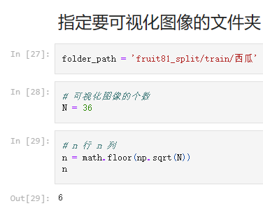

#读取文件夹中的所有图像
images = []
for each_img in os.listdir(folder_path)[:N]:
    img_path = os.path.join(folder_path, each_img)
    img_bgr = cv2.imread(img_path)
    img_rgb = cv2.cvtColor(img_bgr, cv2.COLOR_BGR2RGB)
    images.append(img_rgb)

#画图
fig = plt.figure(figsize=(10, 10))
grid = ImageGrid(fig, 111,  # 类似绘制子图 subplot(111)
                 nrows_ncols=(n, n),  # 创建 n 行 m 列的 axes 网格
                 axes_pad=0.02,  # 网格间距
                 share_all=True
                 )

# 遍历每张图像
for ax, im in zip(grid, images):
    ax.imshow(im)
    ax.axis('off')

plt.tight_layout()
plt.show()