实验一：常规神经网络函数逼近实验

Zza

2023 年 9 月 20  日

1.引言

函数逼近问题是指在不给出函数关系式的前提下， 仅通过大量的函数值对应实例， 对神经网络 进行训练，使得神经网络可以根据一个未知的自变量预测对应的应变量值。

2    实验设计

2.1    实验环境

•  Python 3.9.13

•  NumPy 库

•  神经网络类 NeuralNet（包含前向传播和反向传播方法）

•  均方误差损失函数 mse_loss

2.2    实验参数

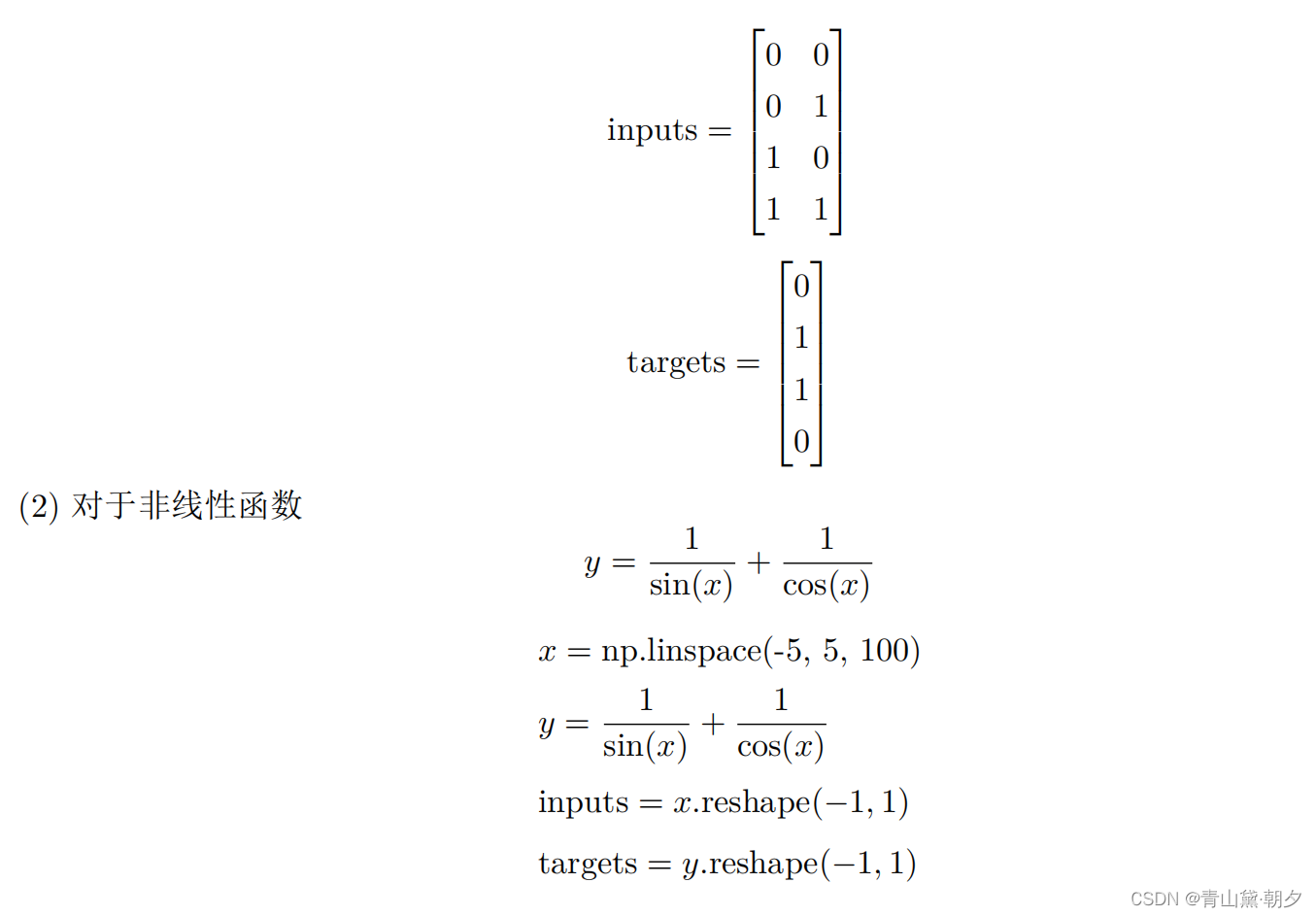
(1) 对于函数 XOR

•  输入层节点数 input__size = 2

•  隐藏层节点数 hidden__size = 18

•  输出层节点数 output__size = 1

•  学习率 learning__rate = 0.01

•  训练迭代次数 num__epochs = 10000

(2) 对于非线性函数

 y = \frac{1}{{\sin(x)}} + \frac{1}{{\cos(x)}} 
 

•  输入层节点数 input__size = 1

•  隐藏层节点数 hidden__size = 100

•  输出层节点数 output__size = 1

•  学习率 learning__rate = 0.01

•  训练迭代次数 num__epochs = 1200000

3    实验步骤

3.1    初始化神经网络模型

model = NeuralNet(input__size, hidden__size, output__size)

3.2    生成输入数据

(1) 对于函数 XOR

  

3.3    训练神经网络模型

for epoch in range(num_epochs):
    # Forward pass
    outputs = model.forward(inputs)
    loss = mse_loss(targets, outputs)
    
    # Backward pass and optimization (SGD)
    model.backward(inputs, targets, outputs, learning_rate)
    
    # Print loss every 1000 epochs
    if (epoch+1) % 1000 == 0:
        print('Epoch [{}/{}], Loss: {:.4f}'.format(epoch+1, num_epochs, loss))

3.4    使用训练好的模型进行预测

(1) 对于 XOR 函数

predicted = (model.forward(inputs) > 0.5).astype(int)

(2)对于非线性函数

 y = \frac{1}{{\sin(x)}} + \frac{1}{{\cos(x)}} 

predicted = model.forward(inputs)

4    实验结果                                                                            3

(1) 对于 XOR 函数经过 10000 次迭代训练后，损失值收敛到 0.00 预测出来的结果为小数，因

此我做了近似

(2) 对于非线性函数

4    实验结果

(1) 对于 XOR 函数经过 10000 次迭代训练后， 损失值收敛到 0.00 预测出来的结果为小数， 因

此我做了近似

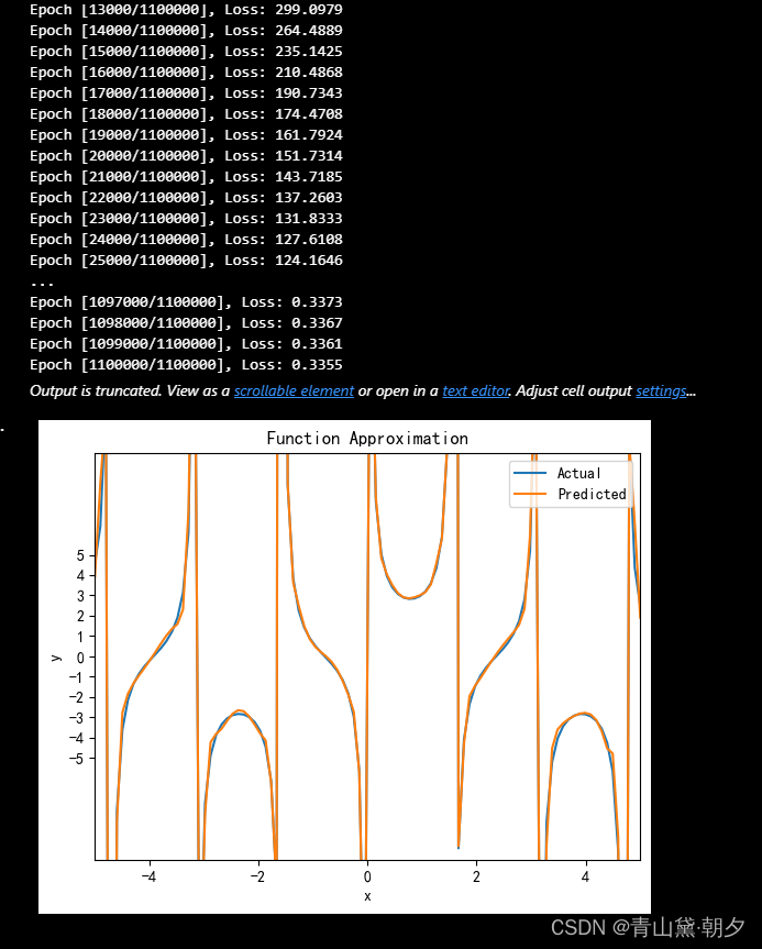
(2) 对于非线性函数

 y = \frac{1}{{\sin(x)}} + \frac{1}{{\cos(x)}} 

经过 120 万次迭代训练后，模型的损失值收敛到 0.2749 ，表明模型在训练数据上取得了良好的拟合 效果。

5    Python Code

import numpy as np

# Define the sigmoid activation function
def sigmoid(x):
    return 1 / (1 + np.exp(-x))

# Define the derivative of the sigmoid function
def sigmoid_derivative(x):
    return x * (1 - x)

# Define the mean squared error loss
def mse_loss(y_true, y_pred):
    return np.mean((y_true - y_pred)**2)

# Define the neural network class
class NeuralNet:
    def __init__(self, input_size, hidden_size, output_size):
        # Initialize weights and biases
        self.weights1 = np.random.randn(input_size, hidden_size)
        self.bias1 = np.zeros((1, hidden_size))
        self.weights2 = np.random.randn(hidden_size, output_size)
        self.bias2 = np.zeros((1, output_size))
    
    def forward(self, x):
        # Perform forward pass
        self.z1 = np.dot(x, self.weights1) + self.bias1
        self.a1 = sigmoid(self.z1)
        self.z2 = np.dot(self.a1, self.weights2) + self.bias2
        self.a2 = self.z2  # Linear activation
        
        return self.a2
    
    def backward(self, x, y, y_pred, learning_rate):
        # Compute gradients
        m = x.shape[0]
        dL_da2 = 2 * (y_pred - y) / m
        dL_dz2 = dL_da2
        dL_dw2 = np.dot(self.a1.T, dL_dz2)
        dL_db2 = np.sum(dL_dz2, axis=0, keepdims=True)
        dL_da1 = np.dot(dL_dz2, self.weights2.T)
        dL_dz1 = dL_da1 * sigmoid_derivative(self.a1)
        dL_dw1 = np.dot(x.T, dL_dz1)
        dL_db1 = np.sum(dL_dz1, axis=0, keepdims=True)
        
        # Update weights and biases
        self.weights1 -= learning_rate * dL_dw1
        self.bias1 -= learning_rate * dL_db1
        self.weights2 -= learning_rate * dL_dw2
        self.bias2 -= learning_rate * dL_db2

input_size = 1
hidden_size = 100
output_size = 1
learning_rate = 0.01
num_epochs = 1100000

# Create neural network model
model = NeuralNet(input_size, hidden_size, output_size)

# Generate input data
x = np.linspace(-5, 5, 100)
y = 1 / np.sin(x) + 1 / np.cos(x)

# Convert inputs and targets to numpy arrays
inputs = x.reshape(-1, 1)  # Assuming you want 100 input features
targets = y.reshape(-1, 1)
# Train the model
for epoch in range(num_epochs):
    # Forward pass
    outputs = model.forward(inputs)
    loss = mse_loss(targets, outputs)
    
    # Backward pass and optimization (SGD)
    model.backward(inputs, targets, outputs, learning_rate)
    
    # Print loss every 1000 epochs
    if (epoch+1) % 1000 == 0:
        print('Epoch [{}/{}], Loss: {:.4f}'.format(epoch+1, num_epochs, loss))

# Predict using the trained model
predicted = model.forward(inputs)

# Plot results (similar to original code)
import matplotlib.pyplot as plt
plt.plot(x, y, label='Actual')
plt.plot(x, predicted, label='Predicted')
plt.xlabel('x')
plt.xlim(-5,5)
plt.ylabel('y')
plt.ylim(-10, 10)
plt.yticks(np.arange(-5, 6, 1))
plt.title('Function Approximation')
plt.legend()
plt.show()

inputs = np.array([[0, 0], [0, 1], [1, 0], [1, 1]])
targets = np.array([[0], [1], [1], [0]])

# Define hyperparameters
input_size = 2
hidden_size = 18
output_size = 1
num_epochs = 10000
learning_rate = 0.01

# Initialize the neural network
model = NeuralNet(input_size, hidden_size, output_size)

# # Training loop
for epoch in range(num_epochs):
    # Forward pass
    outputs = model.forward(inputs)
    loss = mse_loss(targets, outputs)
    
    # Backward pass and optimization (SGD)
    model.backward(inputs, targets, outputs, learning_rate)
    
    # Print loss every 1000 epochs
    if (epoch+1) % 1000 == 0:
        print('Epoch [{}/{}], Loss: {:.4f}'.format(epoch+1, num_epochs, loss))

#Predict using the trained model
predicted = model.forward(inputs)
predicted_I_want = (model.forward(inputs) > 0.5).astype(int)

# Print the predictions
print("Predicted:")
print(predicted)
print("predicted_I_want:")
print(predicted_I_want)
# Print the targets
print("\nTargets:")
print(targets)

7    结论

本实验成功地展示了如何使用反向传播算法来训练神经网络模型， 并对特定数据集进行预测。 通过调整不同的超参数，可以进一步优化模型的性能，以适应不同的任务需求。

训练参数很重要