人工智能（详解机器学习！！！）

人工智能

下图是从一位大佬那拷过来的哦

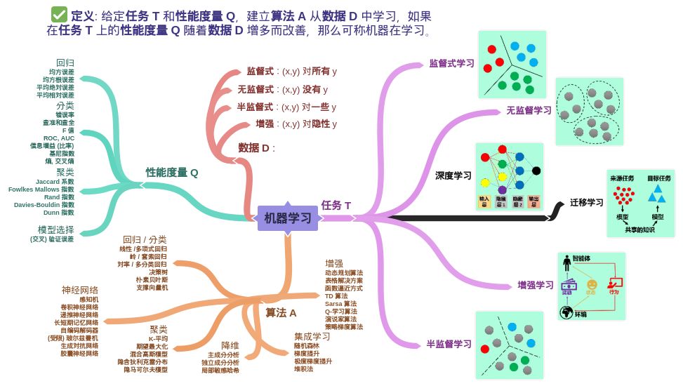
机器学习包含4个元素：数据（经验），任务，性能度量，模型

机器学习的经典定义：利用经验改善系统自身的性能

大数据时代，要得到数据的价值，必须对数据进行有效的数据分析-利用机器学习

|f(x)-y|<=e：f(x)和y近似

P>=1-o：大概率得到f(x)

机器学习：很高的概率得到很好的模型

1.BP

1.1最小二乘法

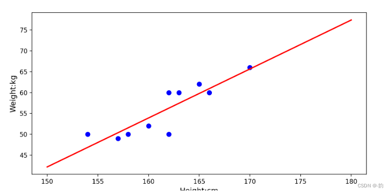
1.拟合曲线：y=kx+b

import numpy as np
import matplotlib.pyplot as plt
import scipy as sp
from scipy.optimize import leastsq

# 样本数据
Xi = np.array([162,160,157,158,162,165,163,170,154,166])
Yi = np.array([50,52,49,50,60,62,60,66,50,60])

# 需要拟合的函数(y=kx+b)
def func(p,x):
    k,b = p
    return k*x+b

# 误差
def error(p,x,y):
    return func(p,x) - y

# 设置初始值
p0 = [1,20]

# 最小二乘函数
Para = leastsq(error,p0,args=(Xi,Yi))
k,b = Para[0]#读取结果

#画样本点
plt.figure(figsize=(8,6))
plt.scatter(Xi,Yi,color='blue',linewidth=2)

# 画线
x = np.linspace(150,180,80)
y = k*x + b

# 绘制线
plt.plot(x,y,color='red',linewidth=2)

# 标签
plt.xlabel('Height:cm',fontsize=12)
plt.ylabel('Weight:kg',fontsize=12)

plt.show()

[外链图片转存失败,源站可能有防盗链机制,建议将图片保存下来直接上传(img-VrUcM54b-1668855606562)(E:%5C%E7%AC%94%E8%AE%B02%5Cimages%5Cimage-20221024203344369.png)]

2.计算残差

残差：真实值与计算值的差别

#最小二乘法
import numpy as np
import matplotlib.pyplot as plt
from statsmodels.graphics.api import qqplot

# 样本数据
Xi = np.array([162,160,157,158,162,165,163,170,154,166])
Yi = np.array([50,52,49,50,60,62,60,66,50,60])
xy_res=[]

# 计算残差函数
def residual(x,y):
    return y - (0.4211697*x-8.2883026)

#循环读取残差
for i in range(0,len(Xi)):
    xy_res.append(residual(Xi[i],Yi[i]))

# 计算残差平方和,和越小效果越好
xy_res_num = np.dot(xy_res,xy_res)

fig = plt.figure(figsize=(8,6))
ax = fig.add_subplot(111)#添加子图
fig = qqplot(np.array(xy_res),line='q',ax=ax)#正态分布

plt.show()

1.2梯度下降法

#梯度下降函数
from numpy import *
import matplotlib.pyplot as plt

# 数据
m = 20#数据集大小
X0 = ones((m,1))
X1 = arange(1,m+1).reshape(m,1)
X = hstack((X0,X1))#堆叠形成数组
Y = array([3,4,5,5,2,4,7,8,11,8,12,11,13,13,16,17,18,17,19,21]).reshape(m,1)
alpha = 0.01#学习率
theta = array([1,1]).reshape(2,1)#theta

# 定义代价函数
def cost_function(theta,x,y):
    diff = dot(x,theta) - y
    return (1/(2*m))*dot(diff.transpose(),diff)

# 定义代价函数对应的梯度函数（代价函数求微）
def gradient_function(theta,x,y):
    diff = dot(x,theta) - y
    return (1/m) * dot(x.transpose(),diff)

# 梯度下降迭代
def gradient_descent(x,y,alpha):
    theta = array([1, 1]).reshape(2, 1)
    gradient = gradient_function(theta,x,y)
    while not all (abs(gradient)<=1e-5):
        theta = theta - alpha*gradient
        gradient = gradient_function(theta, x, y)
    return theta

optimal = gradient_descent(X,Y,alpha)

# 画图
# 散点图
plt.scatter(X1,Y,c="blue",marker="s")
plt.xlabel('X')
plt.ylabel('Y')

# 折线图
x = arange(0,21,0.2)
y = theta[0] + theta[1]*x
plt.plot(x,y,color="red")

plt.show()

2.卷积

2.1 卷积运算

#卷积运算
import struct
import numpy as np
import matplotlib.pyplot as plt

# 矩阵
dateMat = np.ones((7,7))
kernal = np.array([[-1,-1,-1],[-1,8,-1],[-1,-1,-1]])

# 卷积运算函数
def convolve(dateMat,kernal):
    m,n = dateMat.shape
    km,kn = kernal.shape
    newMat = np.ones(((m-km+1),(n-kn+1)))
    tempMat = np.ones((km,kn))
    for row in (m-km+1):
        for col in (n-kn+1):
            for m_k in km:
                for n_k in kn:
                    tempMat[m_k][n_k] = dateMat[row+m_k][col+n_k]*kernal[m_k][n_k]#计算相乘	
        newMat[row][col] = np.sum(tempMat)
    return newMat

2.激活函数

这里举例sigmoid,tanh,relu

#激活函数
import numpy as np
import matplotlib.pyplot as plt
# sigmoid
def sigmoid(x):
    return 1/(1+np.exp(-x))

# tanh
def tanh(x):
    return (np.exp(x) - np.exp(-x))/(np.exp(x)+np.exp(-x))

# reiu
def reiu(x):
    return np.where(x>0,x,0)

x = np.arange(-10,10,0.1)

# 画图
# 创建画布
img = plt.figure()
# 创建子图
s = img.add_subplot(131)
y1 = sigmoid(x)
plt.plot(x,y1,color="red")

t = img.add_subplot(132)
y2 = tanh(x)
plt.plot(x,y2,color="blue")

r = img.add_subplot(133)
y3 = reiu(x)
plt.plot(x,y3,color="green")

plt.show()

2.3池化运算

最大池化

#池化运算（最大池化）
import numpy as np

def pooling(data,m,n):
    a,b = data.shape
    img_new = []
    for i in range(0,a,m):
        line = []#空行
        for j in range(0,b,n):
            x = data[i:i+m,j,j+n]#选区池范围
            line.append(np.max(x))#最大池
        img_new.append(line)
    return img_new
            

池化运算的应用-图像

#池化运算（最大池化）
import matplotlib.pyplot as plt
import numpy as np
from PIL import Image

# 读取图片
img = Image.open("./img/book.jpg")
plt.imshow(img)#绘制热力图
plt.axis('off')#关闭坐标轴

# R，G，B
r,g,b = img.split()
plt.imshow(r)#读取红通道
plt.axis('off')

# 池化函数
def pooling(data,m,n):
    a,b = data.shape
    img_new = []
    for i in range(0,a,m):
        line = []#空行
        for j in range(0,b,n):
            x = data[i:i+m,j:j+n]#选区池范围
            line.append(np.max(x))#最大池
        img_new.append(line)
    return img_new

img_new = pooling(np.array(r),2,2)#2*2的池化区
plt.imshow(img_new)
plt.axis('off')

2.4全连接

normal,larger,smaller

import numpy as np
# 全连接

def sigmoid(x):
    return 1/(1+np.exp(-x))

# 导函数
def sigmoid_derivative(x):
    return sigmoid(x)*(1-sigmoid(x))

# 全连接层
class FullConnectLayer:
#     初始化
    def __init__(self,n_in,n_out,action_func=sigmoid,action_func_der=sigmoid_derivative,flag="normal"):
        self.action_func = action_func#激活函数
        self.action_func_der = action_func_der#激活函数导函数
        self.n_in = n_in#输入层单元数
        self.n_out = n_out#输出层单元个数
        self.init_weight_bias(init_flag=flag)

    def init_weight_bias(self,init_flag):#flag初始化权值和偏置项的标记
        if(init_flag == 'normal'):
#             weight服从N(0,1)分布
            self.weight = np.random.randn(self.n_in,self.n_out)
            self.biase = np.random.randn(self.n_out)
        if(init_flag == 'larger'):
#             weight取值范围（-1，1）
            self.weight = 2 * np.random.randn(self.n_in,self.n_out) - 1 
            self.biase = 2*np.random.randn(self.n_out) - 1
        if(init_flag == 'smaller'):
#             weight取值服从（0，1/x）
            self.weight = np.random.randn(self.n_in,self.n_out/np.sqrt(self.n_out))
            self.biase = np.random.randn(self.n_out)

# 前馈传播
    def __call__(self, input):
        self.input = np.dot(input,self.weight) + self.biase#W*X+b
        output = self.action_func(self.input)
        return output
        

2.5分类函数

softmax

import numpy as np
def softmax(x):
    return np.exp(x) / (np.sum(np.exp(x)))

3.信息熵，交叉熵

3.1信息熵

信息熵：某种特定信息的出现概率，一般而言，当一种信息出现的概率更高时，表明它被传播的更广泛，或者是被引用的程度更高。

信息熵指的是对事件中不确定的信息的度量，其信息熵越大，含有的不确定信息越大。

3.2交叉熵-信息熵最重要的应用

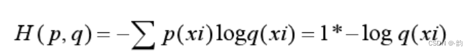
1.交叉熵基本公式

此公式可表示概率分布q(xi)表示概率分布p(xi)的困难程度

交叉熵刻画两个概率分布距离，所得交叉熵值越小，则表示q的分布越接近真实值（与真实值的距离越小）

import numpy as np

# 两个分布
x = np.array([1,0])#p(xi)为真实数据
y = np.array([0.7,0.3])#q(xi)为预测数据

def cross_entropy(y_true,y_pred):
    ce = -(y_true)*np.log(y_pred)#矩阵相乘得到矩阵
    ce = np.mean(ce)#均值得到值
    return ce

print(cross_entropy(x,y))

2.交叉熵的表述

由于在计算交叉熵的时候真实值为0的预测值不参与运算，因此交叉熵公式化简为

设有N种类别，若计算出的[外链图片转存失败,源站可能有防盗链机制,建议将图片保存下来直接上传(img-NcLGAgqj-1668855606565)(E:%5C%E7%AC%94%E8%AE%B02%5Cimages%5Cwps1-1667181269090.png)]>N，则模型无效学习，若<N则学习较好，若=N则没有学习

3.交叉熵的改进1-把无用的利用起来（p(xi)=0）

当p(xi) = 1时，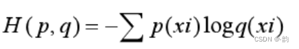

当p(xi) = 0时，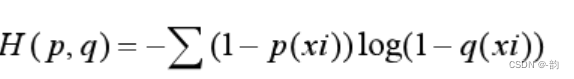

import numpy as np

# 两个分布
x = np.array([1,0])#p(xi)为真实数据
y = np.array([0.7,0.3])#q(xi)为预测数据

def cross_entropy(y_true,y_pred):
    ce_1 = -(y_true)*np.log(y_pred)#y_true=1
    ce_2 = -((1-y_true)*np.log((1-y_pred)))#y_true=0
    ce = ce_1+ce_2#合成
    return np.mean(ce)

print(cross_entropy(x,y))

注：log的值会可能出现nan，所以应该添加截断函数clip(a,min,max)

def cross_entropy(y_true,y_pred):
    ce_1 = -(y_true)*np.log(np.clip(y_pred,1e-10,1))#y_true=1,clip添加截断函数
    ce_2 = -((1-y_true)*np.log(np.clip(1-y_pred,1e-10,1)))#y_true=0
    ce = ce_1+ce_2#合成
    return np.mean(ce)

4.交叉熵的改进2-解决正负样本数量差异过大

定义 alpha = 0…25

当p(xi) = 1时，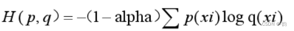

当p(xi) = 0时，

import numpy as np

# 两个分布
x = np.array([1,0])#p(xi)为真实数据
y = np.array([1/100,99/100])#q(xi)为预测数据

def cross_entropy(y_true,y_pred):
    alpha = 0.25
    ce_1 = -(1-alpha)*(y_true)*np.log(np.clip(y_pred,1e-10,1))#y_true=1,clip添加截断函数
    ce_2 = -alpha*((1-y_true)*np.log(np.clip(1-y_pred,1e-10,1)))#y_true=0
    ce = ce_1+ce_2#合成
    return np.mean(ce)

print(cross_entropy(x,y))

5.交叉熵的改进3-解决样本的难易分类

添加权重系数降低权重（1-q(xi)）和q(xi)

定义r=2

当p(xi)=1时，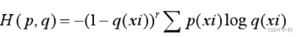

当p(xi)=0时，

import numpy as np

# 两个分布
x = np.array([1,0])#p(xi)为真实数据
y = np.array([0.52,0.76])#q(xi)为预测数据

def cross_entropy(y_true,y_pred):
    r = 1
    ce_1 = -(1-y_pred)*(y_true)*np.log(np.clip(y_pred,1e-10,1))#y_true=1,clip添加截断函数
    ce_2 = -(y_pred)*((1-y_true)*np.log(np.clip(1-y_pred,1e-10,1)))#y_true=0
    ce = ce_1+ce_2#合成
    return np.mean(ce)

print(cross_entropy(x,y))

6.统一交叉熵

alpha=0.25,

r=2

当p(xi)=1时，

当p(xi)=0时，

4.机器学习基本算法

4.1线性回归

线性回归用于拟合回归问题-梯度下降加最小二乘法解决

#线性回归
import numpy as np
import pandas as pd
import matplotlib.pyplot as plt

# 定义误差函数
def liner_loss(w,b,data):#y=wx+b
    x = data[0]
    y = data[1]
    loss = np.sum((y - w*x+b)**2)/data.shape[0]#距离求平方计算误差
    return loss

#梯度
def liner_gradient(w,b,data,a):#a为学习率
#    数据集行数
    N = len(data)
    x = data[0]
    y = data[1]
# 求梯度
    dw = np.sum(-((2/N)*x*(y-w*x+b)))
    db = np.sum(-((2/N)*(y-w*x+b)))
#    更新参数
    w = w-a*dw#梯度下降,方向和上升方向相反
    b = b-a*db
    return w,b

# 梯度下降
def optimer(data,w,b,a,epcoh):#epcoh为训练次数
    for i in range(epcoh):
        w,b = liner_gradient(w,b,data,a)#不断更新
    return w,b

# 绘图
def plot_data(data,w,b):
    x = data[0]
    y = data[1]
    y_predict = w * x + b
    plt.plot(x,y,'o')
    plt.plot(x,y_predict,'k-')
    plt.show()

# 构建模型
def liner_regression():
    data = pd.read_csv('e:/pandas/data.csv', header=None)
    print(len(data))
    print(data.shape[0])
    x = data[0]
    y = data[1]

#     原数据分布
    plt.plot(x,y,"o")
    plt.show()

#     初始化参数
    a = 0.01
    epoch = 100
    w = 0.0
    b = 0.0

#     更新
    w,b = optimer(data,w,b,a,epoch)

#     显示-绘图
    plot_data(data,w,b)

if __name__=='__main__':
    liner_regression()

4.2逻辑回归

逻辑回归用于分类问题，在线性回归的基础上添加sigmoid函数引入非线性元素

注：为了计算概率，逻辑回归的输出范围必须限制在0,1之间，逻辑回归使用sigmoid函数h(z)=1/[z+exp(-z)]，返回0和1之间的数值。

根据y=1以及y=0画出散点图

#sigmoid
def sigmoid(z):
    return 1/(1+np.exp(-z))

# model预测函数
def model(x,theta):
    return sigmoid(np.dot(x,theta.T))

# 损失值
def loss(x,y,theta):
    left = np.multiply(-y,np.log(model(x,theta)))
    right = np.multiply(1-y,np.log((1-model(x,theta))))
    return np.sum((left-right))/len(x)

# 梯度下降函数
def gradient(x,y,theta,alpha,ites):#iters为长度值
    M = len(x)
    cost = np.zeros(ites)
    for i in range(ites):
#         每循环一次，更新参数
        theta = theta - (alpha/M)*(x*(model(x,theta)-y))
        cost[i] = loss(x,y,theta)
    return theta,cost

# 决策边界
def boundary(theta_min,data):
    x1 = np.arange(-4,4,0.01)
    x2 = (theta_min[0,0] + theta_min[0,1]*x1)/(-theta_min[0.2])
    plt = draw_data(data)
    plt.plot(x1,x2)
    plt.show()

4.3决策树

1.流程

策略：分而治之

自根至叶的递归过程，在每一个中间结点寻找一个"划分"属性

停止条件：（1）当前结点包含的样本完全属于同一类别，无需划分

​ （2）当前属性集为空，或是所有样本在所有属性上取值相同，无法划分（没有属性将其分开）

​ （3）当前结点包含的样本集合为空，不能划分。

注：上图来源于周志华教授机器学习初步课程中

2.计算信息熵

import numpy as np

# 两组数据
n_count = 20#产生20个数据
a_list=[]#10个类别
b_list=[]#2个类别
for i in range(n_count):
    a_list.append(np.random.randint(10))
    b_list.append(np.random.randint(2))

# 定义求熵函数
def  entropy_func(data):
    len_data = len(data)#总长度
    entropy = 0
    for i in set(data):#集合不重复
        p = data.count(i)/len_data
        entropy=entropy- p*np.log(p)
    return entropy

entropy_a = entropy_func(a_list)
print(entropy_a)

entropy_b = entropy_func(b_list)
print(entropy_b)

3.其他定义

1.特征熵

在特征A下，求和A的属性的信息熵与其在总数据集中所占的概率的乘积

2.信息增益

不确定性减少越多，信息增益越大

3.信息增益率

4.基尼系数

4.主要代码

# 计算信息熵
def Entropy(dataSet):
    sum = len(dataSet)#总数
    labelCounts = {}#创建一个数据字典，key为最后一列的值
    for a in dataSet:
        currentLabel = a[-1]#取最后一列的值
        if currentLabel not in labelCounts.keys():
            labelCounts[currentLabel] = 0
        labelCounts[currentLabel]+=1#如果存在则加1(计数)
#     计算信息熵
    for k in labelCounts:
        prob = float(labelCounts[k])/sum
        entropy = entropy - prob * np.log(prob)
    return entropy

# 按指定的特征划分数据，返回数据集(OutLook = 'sunny')
def splitDataSet(dataSet,i,value):#i为循环的列号(特征),value为特征值
    rets = []#存放value值所在的行里除value值外的其他值
    for a in dataSet:
        if(a[i] == value):#遍历a[i]列，找到value
            ret = a[:i]
            ret.extend[i+1:]
            rets.append(ret)
    return rets

# 选取当前数据集下，用于划分数据集的最优特征
def chooseBestFeature(dataSet):
    FeatureCounts = len(dataSet[0] - 1)#特征个数
    baseEntropy = chooseBestFeature(dataSet)#计算当前信息熵
    bestGain = 0.0#初始化信息增益
    bestFeature = -1#初始化最优特征
    for i in range(FeatureCounts):#遍历特征
        featureValues = [example[i] for example in dataSet]#获得特征值
        uniqueValues = set(featureValues)
        newEntropy = 0.0
        for value in uniqueValues:#遍历特征值
            subDataSet = splitDataSet(dataSet,i,value)#获得特征值自己的数据集
            prob = len(subDataSet)/float(len(dataSet))
            newEntroy = newEntroy + prob * Entropy(subDataSet)#特征值的熵之和=特征熵
        infoGain = newEntropy - baseEntropy#计算信息增益
        if(infoGain>bestGain):
            bestGain = infoGain
            bestFeature = i
    return bestFeature

5.剪枝

剪枝方法和程度对决策树泛化性能的影响更为显著

剪枝-过拟合

基本策略：（1）预剪枝：提前终止某些分支的生长

​ （2）后剪枝：生成一棵完全树，再“回头”剪枝

基本思路：样本赋权，权重划分

计算有值的信息增益，然后用信息增益*权重（值的个数/总数），更新信息增益。

4.4主成分分析

1.步骤

(1)将矩阵去中心化，得到矩阵B（对于所有样本，每一个特征都减去自己的均值）

(2)构建协方差矩阵

(3)求解协方差矩阵C的特征值以及特征向量

(4)将特征向量按照特征由大到小进行排序，取前k（前k个特征和占所有特征和的0.85）个特征向量组成矩阵U

(5)
即为降维到k维后的特征向量空间

2.其他定义

特征值贡献度：前k个特征和占所有特征和的比值

3.代码实现

import numpy as np
from numpy.linalg import eig
from sklearn.datasets import load_iris

# 鸢尾花数据集实现pca
def pca(X,k):
    X = X - X.mean(axis=0)#X向量去中心化
    X_cov = np.cov(X.T,ddof=0)#计算X的协方差矩阵,自由度可以选择0或1(np.dot((X-u).T,(X-u))/X.shape[0])
    eig_value,eig_vector = eig(X_cov)#计算协方差矩阵的特征值和特征向量
    k_index = np.argsort(eig_value)[-k:][::-1]#得到最大的k个特征值的索引(升序后取后k个再倒叙)
    k_eig_vec = eig_vector[k_index]#取对应的特征值（U）
    return np.dot(X,k_eig_vec.T)#返回X与U的转置相乘

# 初始化数据
X = load_iris().data
k = 2
X_pca = pca(X,k)
print(X_pca)

4.5线性判别分析

步骤：

1.计算类内散度矩阵Sw,类间散度矩阵Sb

2.w = Sw的逆*(mu1-mu2)（mu1表示1类数据集的均值向量）

3.y=w的转置*x

#LDA线性判别分析代码
import numpy  as np
from sklearn.datasets import  load_iris
import matplotlib.pyplot as plt


# LDA
def LDA(X,Y):
    X1 = [X[i] for i in range(len(X)) if Y[i] == 0]
    X2 = [X[i] for i in range(len(X)) if Y[i] == 1]

    len1 = len(X1)
    len2 = len(X2)

    # 得到y1,y2
    Y1 = [1 for i in range(len1)]
    Y2 = [2 for i in range(len2)]

    # 求解mu1,mu2
    mu1 = np.mean(X1,axis=0)
    mu2 = np.mean(X2,axis=0)

    # 求解sw
    cov1 = np.dot((X1-mu1).T,(X1-mu1))
    cov2 = np.dot((X2-mu2).T,(X2-mu2))
    sw = cov1+cov2

    # 求解w
    w = np.dot(np.linalg.inv(sw),(mu1-mu2)).reshape(-1,1)
    print(w)
    X1_new = funx(X1,w)
    X2_new = funx(X2,w)
    return X1_new,X2_new,Y1,Y2

def funx(x,w):
    return np.dot((x),w)

# 初始化数据
if '__main__'==__name__:
    iris = load_iris()
    X = iris.data
    Y = iris.target
    
    X1,X2,Y1,Y2 = LDA(X,Y)

    # 原图像
    plt.scatter(X[:, 0], X[:, 1], marker='o', c=Y)
    plt.show()
	#现图像
    plt.plot(X1,Y1,'b*')
    plt.plot(X2,Y2,'ro')
    plt.show()

4.6朴素贝叶斯

1.定义

贝叶斯决策理论的核心思想：选择具有最高概率的决策

朴素贝叶斯：假设各个特征相互独立

2.步骤

1.计算每个类别的概率p(Y=c)

2.计算每个类别下每个特征的条件概率p(X=x|Y=c)

3.计算

3.代码实现

#朴素贝叶斯
import numpy as np
# 创建实验样本
def createSample():
    wordList = [['my', 'dog', 'has', 'flea', 'problems', 'help', 'please'],
                   ['maybe', 'not', 'take', 'him', 'to', 'dog', 'park', 'stupid'],
                   ['my', 'dalmation', 'is', 'so', 'cute', 'I', 'love', 'him'],
                   ['stop', 'posting', 'stupid', 'worthless', 'garbage'],
                   ['mr', 'licks', 'ate', 'my', 'steak', 'how', 'to', 'stop', 'him'],
                   ['quit', 'buying', 'worthless', 'dog', 'food', 'stupid']]
    classVec = [1,0,1,0,0,1]#标签向量
    return wordList,classVec

# 创建不重复词汇的列表
def createVocablist(wordList):
    words = set([])
    for word in wordList:
        words = words | set(word)#创建两个集合的并集
    return list(words)

# 输出文档向量-表示词汇表中的单词是否在输入文档中出现
def setWordVec(words,inputList):
    wordVec = [0]*len(words)
    for word in inputList:
        if word in words:
            wordVec[words.index(word)] = 1
        else:
            print("单词 %s 不在词汇表中" %word)
    return wordVec


# 朴素贝叶斯训练函数
def trainNBO(trainMatrix,trainCategory):

    pAbusive = sum(trainCategory)/len(trainCategory)#求侮辱类的概率
    numWords = len(trainMatrix[0])#每篇文档总词数
    numDos = len(trainMatrix)#文档总数

    p0 = np.zeros(numWords)
    p1 = np.zeros(numWords)

    p0D = 0.0#初始化概率
    p1D = 0.0

    for i in range(numDos):
        if(trainCategory[i] == 1):
            p0+=trainMatrix[i]#向量相加
            p0D+=sum(trainMatrix[i])
        else:
            p1 += trainMatrix[i]  # 向量相加
            p1D += sum(trainMatrix[i])
    p0V = p0/p0D
    p1V = p1/p1D
    return p0V,p1V,pAbusive

# 测试函数效果

# 创建实验样本
listPosts, listClasses = createSample()
print('数据集\n', listPosts)

# 创建词汇表
myVocabList = createVocablist(listPosts)
print('词汇表:\n', myVocabList)

trainMat = []

# 输出文档向量
for list in listPosts:
    trainMat.append(setWordVec(myVocabList,list))

# 贝叶斯
p0V,p1V,pAb = trainNBO(trainMat,listClasses)

print('p0V:\n', p0V)
print('p1V:\n', p1V)
print('pAb:\n', pAb)

4.7集成方法

注：以下部分资料来源于sklearn官方文档

集成方法 的目标是把多个使用给定学习算法构建的基估计器的预测结果结合起来，从而获得比单个估计器更好的泛化能力/鲁棒性。

1.Bagging

bagging 方法有很多种，其主要区别在于随机抽取训练子集的方法不同：

• 如果抽取的数据集的随机子集是样例的随机子集，我们叫做粘贴 (Pasting) [B1999] 。
• 如果样例抽取是有放回的，我们称为 Bagging [B1996] 。
• 如果抽取的数据集的随机子集是特征的随机子集，我们叫做随机子空间 (Random Subspaces) [H1998] 。
• 最后，如果基估计器构建在对于样本和特征抽取的子集之上时，我们叫做随机补丁 (Random Patches)

from sklearn.ensemble  import BaggingClassifier
from sklearn.neighbors import KNeighborsClassifier
#构建一个KNeighborsClassifier估计器的bagging实例
bagger = BaggingClassifier(KNeighborsClassifier(),max_samples=0.5,max_features=0.5)

max_samples控制样例大小，max_features控制特征大小，bootstrap控制样例的抽取是否可放回

2.随机森林

sklearn.ensemble 模块包含两个基于 随机决策树 的平均算法： RandomForest 算法和 Extra-Trees 算法。 这两种算法都是专门为树而设计的扰动和组合技术（perturb-and-combine techniques） [B1998] 。 这种技术通过在分类器构造过程中引入随机性来创建一组不同的分类器。集成分类器的预测结果就是单个分类器预测结果的平均值。

from sklearn.ensemble import RandomForestClassifier
X = [[0,0],[1,1]]#训练样本的数组[n_samples,n_features]
Y = [0,1]#训练样本目标值的数组
clf = RandomForestClassifier(n_estimators=10)#几棵树
clf = clf.fit(X,Y)

n_estimators:森林中树木的数量

criterion : { “squared_error”, “absolute_error”, “poisson”}, default=“squared_error”
标准：{“平方误差”、“绝对误差”、“泊松”}、默认=“平方误差”（测量分割质量的功能）

max_depth:树的最大深度

min_samples_split:拆分内部结点所需的最小样本数

min_samples_leaf:一个叶节点所需的最小样本数

min_weight_fraction_leaf:一个叶子节点处所有输入样本的权重之和的最小加权分数

max_features:在寻找最佳拆分时要考虑的功能数量

max_leaf_nodes:最大叶子结点

min_impurity_decrease:最小杂质减少

bootstrap:创建树时是否使用引导示例，如果为false则整个数据集用于构建每个树

oob_score:是否使用带包的样本来估计泛化分数，只有在引导=真的情况才可用

n_jobs:

random_state:随机状态

ccp_alpha:用于最小成本复杂度的复杂度参数，成本最大的子树

max_samples:最大样本数

随机森林构建过程的随机性能够产生具有不同预测错误的决策树。通过取这些决策树的平均，能够消除部分错误。随机森林虽然能够通过组合不同的树降低方差，但是有时会略微增加偏差。

from sklearn.datasets import load_iris
from sklearn.ensemble import RandomForestClassifier

iris = load_iris()
rf  = RandomForestClassifier()#默认
X = iris.data[:150]
Y = iris.target[:150]
rf.fit(X,Y)
# 预测样本
instance = iris.data[[50]]
print("预测类别",rf.predict(instance),"真实类别",iris.target[50])
instance = iris.data[[140]]
print("预测类别",rf.predict(instance),"真实类别",iris.target[140])

3.AdaBoot算法（迭代）----------boosting

AdaBoost 的核心思想是用反复修改的数据（校对者注：主要是修正数据的权重-----提高那些被前一轮弱分类器错误分类的样本的权值，降低那些被正确分类的样本的权值）来训练一系列的弱学习器(一个弱学习器模型仅仅比随机猜测好一点, 比如一个简单的决策树),由这些弱学习器的预测结果通过加权投票(或加权求和)的方式组合, 得到我们最终的预测结果。

1.步骤：

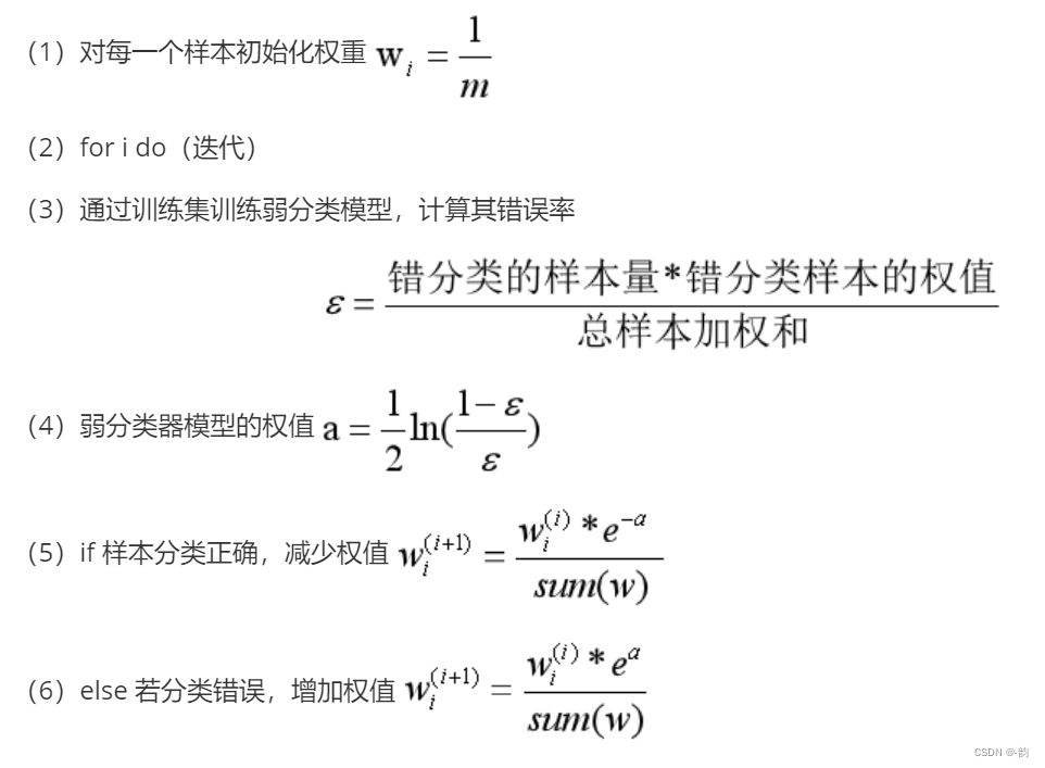
​ 公式推导：

​

2.参数说明

base_estimator:基分类器，默认是决策树，在该分类器基础上进行boosting，理论上可以是任意一个分类器，但是如果是其他分类器时需要指明样本权重。

n_estimators:基分类器提升（循环）次数，默认是50次，这个值过大，模型容易过拟合；值过小，模型容易欠拟合。

learning_rate:学习率，表示梯度收敛速度，默认为1，如果过大，容易错过最优值，如果过小，则收敛速度会很慢；该值需要和n_estimators进行一个权衡，当分类器迭代次数较少时，学习率可以小一些，当迭代次数较多时，学习率可以适当放大。

获取一个好的预测结果主要需要调整的参数是 n_estimators 和 base_estimator 的复杂度

4.8 k-means聚类

1.定义

K均值聚类（k-means）是基于样本集合划分的聚类算法。K均值聚类将样本集合划分为k个子集，构成k个类，将n个样本分到k个类中，每个样本到其所属类的中心距离最小，每个样本仅属于一个类，这就是k均值聚类。

2.步骤

（1）初始化选择k个样本中心

（2）计算每个样本到各个样本中心的距离，分别选择最小的距离进行聚类

（3）分别计算每个聚类的质心，重新计算每个样本到每个新的质心的距离，重新进行聚类

（4）若聚类后聚类结果不变，则直接输出，若发生变化，则循环（2）（3），直到聚类结果不发生变化

3.实例代码

n_cluster：聚类数

labels_：标签

cluster_centers_：聚类中心

import numpy as np
from sklearn.datasets import load_iris
from sklearn.model_selection import train_test_split
import matplotlib.pyplot as plt
from sklearn.cluster import KMeans

iris = load_iris()
X = iris.data[:,2:4]
Y = iris.target
print(iris.feature_names)

# 划分训练集与测试集
X_train,X_test,Y_train,Y_test = train_test_split(X,Y,test_size=0.3,random_state=42)

# 散点图
plt.scatter(X[:,0],X[:,1],c="blue",marker="o",label='iris')
plt.xlabel('petal length (cm)')
plt.ylabel('petal width (cm)')
plt.legend(loc='upper left')
plt.show()

# 开始聚类
estimater = KMeans(n_clusters=3)#构造聚类器,划分为3类
estimater.fit(X_train)#训练样本
label_pred = estimater.labels_#获取标签
print(label_pred)#0 1 2
print(estimater.cluster_centers_)#聚类中心

# 分类-训练集
X0 = X_train[label_pred == 0]
X1 = X_train[label_pred == 1]
X2 = X_train[label_pred == 2]
plt.scatter(X0[:,0],X0[:,1],c="red",marker="o",label='label0')
plt.scatter(X1[:,0],X1[:,1],c="blue",marker="*",label='label1')
plt.scatter(X2[:,0],X2[:,1],c="green",marker="+",label='label2')
plt.xlabel('petal length (cm)')
plt.ylabel('petal width (cm)')
plt.legend(loc='upper left')
plt.show()

# 测试测试集属于哪一类
print(estimater.predict(X_test))
# 绘制测试集
predict_0 = X_test[estimater.predict(X_test) == 0]
predict_1 = X_test[estimater.predict(X_test) == 1]
predict_2 = X_test[estimater.predict(X_test) == 2]
plt.scatter(predict_0[:,0],predict_0[:,1],c="tomato",marker="o",label="predict0")
plt.scatter(predict_1[:,0],predict_1[:,1],c="skyblue",marker="*",label="predict1")
plt.scatter(predict_2[:,0],predict_2[:,1],c="greenyellow",marker="+",label="predict2")
plt.xlabel('petal length (cm)')
plt.ylabel('petal width (cm)')
plt.legend()
plt.show()

原始数据散点图

训练集聚类图

测试集聚类图

4.9k最近邻

1.定义

为了判定未知样本的类别，以全部训练样本作为代表点，计算未知样本与所有训练样本的距离，并以最近邻者的类别作为决策未知样本类别的唯一依据

2.步骤

（1）计算测试集与训练集的欧式距离

（2）将距离以升序的方式排序

（3）选取前k个一直类别数据集的数据

（4）统计前k个数据所属不同类别出现的频数

（5）频数最大的类别的标签作为测试集的标签

3.代码

import numpy as np
import matplotlib.pyplot as plt
from math import sqrt

# 准备数据
data = [[1,0.9],[1,1],[0.1,0.2],[0,0.1]]
labels = ['A','A','B','B']
test = [[0.1,0.3]]
print(type(data))
# 绘制原始数据图
for i in range(len(data)):
    print(data[i])
    plt.scatter(data[i][0],data[i][1],c="red",marker="o")
plt.scatter(test[0][0],test[0][1],c="blue",marker="*")
plt.show()

# 计算测试集与训练集的距离
distance = []
label = []
for i in range(len(data)):
    d = 0
    d = sqrt((test[0][0]-data[i][0])**2+(test[0][1]-data[i][1])**2)
    distance.append(d)
    label.append(i)#下标
print(distance)

# 升序,取前三个
for i in range(len(data)-1):
    for j in range(i+1,len(data)):
        if(distance[i] > distance[j]):
            distance[i],distance[j] = distance[j],distance[i]
            label[i],label[j] = label[j],label[i]
print("排序后:",distance)
print("取前三个:",distance[:3])

# 根据标签计算频数
A = 0
B = 0
for i in range(len(label[:3])):
    if(labels[label[i]] == 'A'):
        A += 1
    else:
        B += 1
print("A的数量",A)
print("B的数量",B)
print("计算结果与图中一致")

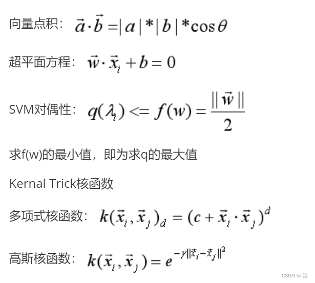
4.10支持向量机

1.定义

支持向量机是一种分类器，对于做出标记的两组向量，给出一个最优分割超曲面把这两组向量分割到两边，使得两组向量中离此超平面最近的向量（即所谓支持向量）到此超平面的距离都尽可能远。（引用）

2.数学知识储备

3.实现代码

#支持向量机
import matplotlib.pyplot as plt
import numpy as np
from sklearn import datasets,linear_model,model_selection,svm

# 数据分类
def load_data_classfication():
    iris = datasets.load_iris
    x_train = iris.data
    y_train = iris.target
    return model_selection.train_test_split(x_train,y_train,test_size=0.2,random_state=0,stratify=y_train)

# 线性核
'''
    coef_:各个特征权重
    intercept_:截距
    score(x,y):返回在（x,y）上的预测准确率
'''
def test_SVC_linear(*data):
    x_train,x_test,y_train,y_test = data
    cls =  svm.SVC(kernel='linear')
    cls.fit(x_train,y_train)
    print('Coefficients:%s.intercept %s' % (cls.coef_, cls.intercept_))
    print('Score:%.2f' % cls.score(x_test, y_test))

# 多形式核
'''
    degree:多项式核函数的系数
    gamma:核函数的系数（'rbf','sigmoid','poly'）
    coef0:指定该函数的自由项('poly','sigmoid')
'''
def test_SVC_poly(*data):
    x_train,x_test,y_train,y_test = data
    fig = plt.figure()

    degrees = range(1,20)
    train_scores = []
    test_scores = []
    for degree in degrees:
        cls = svm.SVC(kernel='poly',degree=degree)
        cls.fit(x_train,y_train)
        train_scores.append(cls.score(x_train,y_train))
        test_scores.append(cls.score(x_test,y_test))
    ax = fig.add_subplot(1,3,1)
    ax.plot(degree,train_scores,label='Training score',marker="o")
    ax.plot(degree, test_scores, label='Testing score', marker="+")
    ax.set_title('SVC_poly_degree')
    ax.set_xlabel('p')
    ax.set_ylabel('score')
    ax.set_ylim(0, 1.05)
    ax.legend(loc='best', framealpha=0.5)

    gammas = range(1,20)
    train_scores = []
    test_scores = []
    for gamma in gammas:
        cls = svm.SVC(kernel='poly',gamma=gamma,degree=3)
        cls.fit(x_train,y_train)
        train_scores.append(cls.score(x_train, y_train))
        test_scores.append(cls.score(x_test, y_test))
    ax = fig.add_subplot(1, 3, 2)
    ax.plot(gamma, train_scores, label='Training score', marker="o")
    ax.plot(gamma, test_scores, label='Testing score', marker="+")
    ax.set_title('SVC_poly_gamma')
    ax.set_xlabel(r'$\gamma$')
    ax.set_ylabel('score')
    ax.set_ylim(0, 1.05)
    ax.legend(loc='best', framealpha=0.5)

    rs = range(1,20)
    train_scores = []
    test_scores = []
    for r in rs:
        cls = svm.SVC(kernel='poly',coef0=r ,gamma=10, degree=3)
        cls.fit(x_train, y_train)
        train_scores.append(cls.score(x_train, y_train))
        test_scores.append(cls.score(x_test, y_test))
    ax = fig.add_subplot(1, 3, 3)
    ax.plot(gamma, train_scores, label='Training score', marker="o")
    ax.plot(gamma, test_scores, label='Testing score', marker="+")
    ax.set_title('SVC_poly_r')
    ax.set_xlabel(r'$\r')
    ax.set_ylabel('score')
    ax.set_ylim(0, 1.05)
    ax.legend(loc='best', framealpha=0.5)

if __name__ == "__main__":
    x_train,x_test,y_train,y_test=load_data_classfication()
    test_SVC_linear(x_train,x_test,y_train,y_test)
    test_SVC_poly(x_train,x_test,y_train,y_test)

4.解的特性

训练完成后，最终模型仅与支持向量有关

5.特征空间映射

将样本从原始空间映射到一个更高维的特征空间，使样本在这个特征空间内线性可分

6.核函数

绕过显式考虑特征映射，以及计算高维内积的困难

Mercer定理：若一个对称函数所对应的核矩阵半正定，则它就能作为核函数使用

上图来源周志华教授“机器学习初步“

5、模型评估与选择

解决的问题

1.泛化误差：在”未来“样本上的误差

2.经验误差：在巡练集上的误差

机器学习的算法与技术都是为了：缓解过拟合问题

3.三个关键问题：

（1）如何获得测试结果：评估方法

（2）如何评估性能优劣：性能度量

（3）如何判断实质差别：比较检验

1.评估方法

关键：怎么获得测试集

测试集应该与训练集互斥

常见方法：留出法

​ 交叉验证法

​ 自助法（有放回采样）

调参与最终模型

算法的参数：一般由人工设定，亦称”超参数“

模型的参数：一般由学习确定

调参：先产生若干模型，然后基于评估方法进行选择

调参数就是在进行模型选择

区别：验证集：训练集中专门留出来用于调参数的部分

​ 测试集：看模型的性能

算法参数选定后，要用”训练集”+“验证集”重新训练最终模型

2.性能度量

性能度量是衡量模型泛化能力的评价标注，反映了任务需求

回归任务常使用均方误差

分类：错误率，精度

3.比较检验

常用方法：统计假设检验