Matplotlib学习日记(五)

学习目标：

不同类型图像绘制2

学习内容：

面积图
面积图是在折线图的基础下将下面部分填满颜色

x = [1,2,3,4,5]
y = np.random.randint(10,100,5)

plt.stackplot(x,y)

成品:

热力图

# ===================随机生成数据=======================
df = pd.DataFrame({
    "省份":["广东","广西","湖南","湖北","江西","四川","福建","江苏","河南","河北","山东","山西"],
    "产品A":np.random.randint(4600,10000,12),
    "产品B":np.random.randint(4600,10000,12),
    "产品C":np.random.randint(4600,10000,12),
    "产品D":np.random.randint(4600,10000,12),
    "产品E":np.random.randint(4600,10000,12),
    "产品F":np.random.randint(4600,10000,12),
    "产品G":np.random.randint(4600,10000,12),
})
# =====================将数据分开=======================
y = df.省份
x = df.drop(columns="省份").columns
# 绘制热力图
plt.figure(figsize=(8,10))

# ========================热力图=======================
plt.imshow(data,
           cmap="Blues" # 颜色映射
           )

# 修改刻度
plt.xticks(range(len(x)) # 位置
           ,x            # 值
)
plt.yticks(range(len(y))
           ,y
           )

for i in range(len(x)):
    for j in range(len(y)):
        plt.text(i,j,data[j][i],ha="center",va="center")

# 显示颜色条
plt.colorbar()

成品:

极坐标图

N = 8
x = np.linspace(0,2*np.pi,N,endpoint=False)
height = np.random.randint(3,15,size=8)

width = 2*np.pi/N

axes = plt.subplot(111,projection="polar")
axes.bar(x,height,width,bottom=0,color=np.random.rand(8,3))

雷达图

plt.figure(figsize=(5,5))

x = np.linspace(0,2*np.pi,6,endpoint=False)
x = np.concatenate((x,[x[0]]))
y = [80,60,90,70,75,100]
y = np.concatenate((y,[y[0]]))
axes = plt.subplot(111,polar=True)

axes.plot(x,y,"o-",lw=2)
axes.fill(x,y,color="r",alpha=0.3)

axes.set_rgrids([20,40,60,80,100],fontsize=12)

成品:

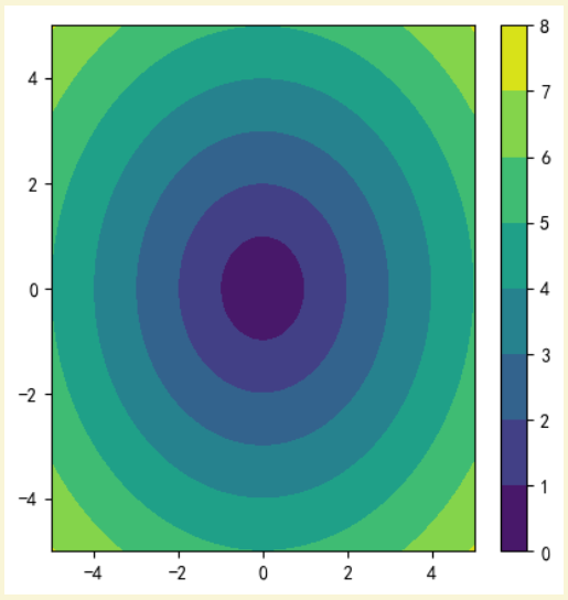
等高线图

plt.figure(figsize=(5,5))
x = np.linspace(-5,5,100)
y = np.linspace(-5,5,100)

x,y = np.meshgrid(x,y)

Z = np.sqrt(x*x+y*y)

cb = plt.contourf(x,y,Z)
plt.colorbar(cb)

成品:

图片处理

img = plt.imread("图片位置")
# 显示图片
plt.imshow(img)
# 垂直反转
plt.imshow(img,origin="lower")
# 左右反转
plt.imshow(img[:,::-1])
# 截取部分
plt.imshow(img[上行:下行,左列:右列])
# 保存图片
plt.imsave("图片地址",img)