


目录
一、实现卷积-池化-激活
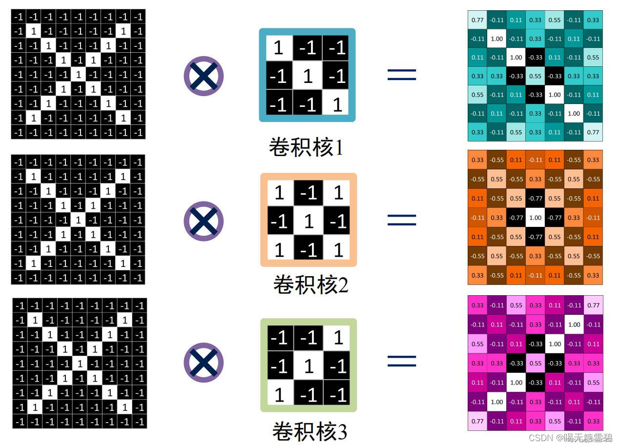
1. Numpy版本:手工实现 卷积-池化-激活
自定义卷积算子,池化算子实现:
代码如下:
运行结果:
x=
 [[-1 -1 -1 -1 -1 -1 -1 -1 -1]
 [-1  1 -1 -1 -1 -1 -1  1 -1]
 [-1 -1  1 -1 -1 -1  1 -1 -1]
 [-1 -1 -1  1 -1  1 -1 -1 -1]
 [-1 -1 -1 -1  1 -1 -1 -1 -1]
 [-1 -1 -1  1 -1  1 -1 -1 -1]
 [-1 -1  1 -1 -1 -1  1 -1 -1]
 [-1  1 -1 -1 -1 -1 -1  1 -1]
 [-1 -1 -1 -1 -1 -1 -1 -1 -1]]
feature_map:
 [[[ 0.78 -0.11  0.11  0.33  0.56 -0.11  0.33]
  [-0.11  1.   -0.11  0.33 -0.11  0.11 -0.11]
  [ 0.11 -0.11  1.   -0.33  0.11 -0.11  0.56]
  [ 0.33  0.33 -0.33  0.56 -0.33  0.33  0.33]
  [ 0.56 -0.11  0.11 -0.33  1.   -0.11  0.11]
  [-0.11  0.11 -0.11  0.33 -0.11  1.   -0.11]
  [ 0.33 -0.11  0.56  0.33  0.11 -0.11  0.78]]

 [[ 0.33 -0.56  0.11 -0.11  0.11 -0.56  0.33]
  [-0.56  0.56 -0.56  0.33 -0.56  0.56 -0.56]
  [ 0.11 -0.56  0.56 -0.78  0.56 -0.56  0.11]
  [-0.11  0.33 -0.78  1.   -0.78  0.33 -0.11]
  [ 0.11 -0.56  0.56 -0.78  0.56 -0.56  0.11]
  [-0.56  0.56 -0.56  0.33 -0.56  0.56 -0.56]
  [ 0.33 -0.56  0.11 -0.11  0.11 -0.56  0.33]]

 [[ 0.33 -0.11  0.56  0.33  0.11 -0.11  0.78]
  [-0.11  0.11 -0.11  0.33 -0.11  1.   -0.11]
  [ 0.56 -0.11  0.11 -0.33  1.   -0.11  0.11]
  [ 0.33  0.33 -0.33  0.56 -0.33  0.33  0.33]
  [ 0.11 -0.11  1.   -0.33  0.11 -0.11  0.56]
  [-0.11  1.   -0.11  0.33 -0.11  0.11 -0.11]
  [ 0.78 -0.11  0.11  0.33  0.56 -0.11  0.33]]]
pooling:
 [[1.   0.33 0.56 0.33]
 [0.33 1.   0.33 0.56]
 [0.56 0.33 1.   0.11]
 [0.33 0.56 0.11 0.78]]
pooling:
 [[0.56 0.33 0.56 0.33]
 [0.33 1.   0.56 0.11]
 [0.56 0.56 0.56 0.11]
 [0.33 0.11 0.11 0.33]]
pooling:
 [[0.33 0.56 1.   0.78]
 [0.56 0.56 1.   0.33]
 [1.   1.   0.11 0.56]
 [0.78 0.33 0.56 0.33]]
relu map :
 [[0.78 0.   0.11 0.33 0.56 0.   0.33]
 [0.   1.   0.   0.33 0.   0.11 0.  ]
 [0.11 0.   1.   0.   0.11 0.   0.56]
 [0.33 0.33 0.   0.56 0.   0.33 0.33]
 [0.56 0.   0.11 0.   1.   0.   0.11]
 [0.   0.11 0.   0.33 0.   1.   0.  ]
 [0.33 0.   0.56 0.33 0.11 0.   0.78]]
relu map :
 [[0.33 0.   0.11 0.   0.11 0.   0.33]
 [0.   0.56 0.   0.33 0.   0.56 0.  ]
 [0.11 0.   0.56 0.   0.56 0.   0.11]
 [0.   0.33 0.   1.   0.   0.33 0.  ]
 [0.11 0.   0.56 0.   0.56 0.   0.11]
 [0.   0.56 0.   0.33 0.   0.56 0.  ]
 [0.33 0.   0.11 0.   0.11 0.   0.33]]
relu map :
 [[0.33 0.   0.56 0.33 0.11 0.   0.78]
 [0.   0.11 0.   0.33 0.   1.   0.  ]
 [0.56 0.   0.11 0.   1.   0.   0.11]
 [0.33 0.33 0.   0.56 0.   0.33 0.33]
 [0.11 0.   1.   0.   0.11 0.   0.56]
 [0.   1.   0.   0.33 0.   0.11 0.  ]
 [0.78 0.   0.11 0.33 0.56 0.   0.33]]
2. Pytorch版本:调用函数实现 卷积-池化-激活
调用框架自带算子实现,对比自定义算子
代码如下:
import torch
import torch.nn as nn

x = torch.tensor([[[[-1, -1, -1, -1, -1, -1, -1, -1, -1],
                    [-1, 1, -1, -1, -1, -1, -1, 1, -1],
                    [-1, -1, 1, -1, -1, -1, 1, -1, -1],
                    [-1, -1, -1, 1, -1, 1, -1, -1, -1],
                    [-1, -1, -1, -1, 1, -1, -1, -1, -1],
                    [-1, -1, -1, 1, -1, 1, -1, -1, -1],
                    [-1, -1, 1, -1, -1, -1, 1, -1, -1],
                    [-1, 1, -1, -1, -1, -1, -1, 1, -1],
                    [-1, -1, -1, -1, -1, -1, -1, -1, -1]]]], dtype=torch.float)
print(x.shape)
print(x)

print("--------------- 卷积  ---------------")
conv1 = nn.Conv2d(1, 1, (3, 3), 1)  # in_channel , out_channel , kennel_size , stride
conv1.weight.data = torch.Tensor([[[[1, -1, -1],
                                    [-1, 1, -1],
                                    [-1, -1, 1]]
                                   ]])
conv2 = nn.Conv2d(1, 1, (3, 3), 1)  # in_channel , out_channel , kennel_size , stride
conv2.weight.data = torch.Tensor([[[[1, -1, 1],
                                    [-1, 1, -1],
                                    [1, -1, 1]]
                                   ]])
conv3 = nn.Conv2d(1, 1, (3, 3), 1)  # in_channel , out_channel , kennel_size , stride
conv3.weight.data = torch.Tensor([[[[-1, -1, 1],
                                    [-1, 1, -1],
                                    [1, -1, -1]]
                                   ]])

feature_map1 = conv1(x)
feature_map2 = conv2(x)
feature_map3 = conv3(x)

print(feature_map1 / 9)
print(feature_map2 / 9)
print(feature_map3 / 9)

print("--------------- 池化  ---------------")
max_pool = nn.MaxPool2d(2, padding=0, stride=2)  # Pooling
zeroPad = nn.ZeroPad2d(padding=(0, 1, 0, 1))  # pad 0 , Left Right Up Down

feature_map_pad_0_1 = zeroPad(feature_map1)
feature_pool_1 = max_pool(feature_map_pad_0_1)
feature_map_pad_0_2 = zeroPad(feature_map2)
feature_pool_2 = max_pool(feature_map_pad_0_2)
feature_map_pad_0_3 = zeroPad(feature_map3)
feature_pool_3 = max_pool(feature_map_pad_0_3)

print(feature_pool_1.size())
print(feature_pool_1 / 9)
print(feature_pool_2 / 9)
print(feature_pool_3 / 9)

print("--------------- 激活  ---------------")
activation_function = nn.ReLU()

feature_relu1 = activation_function(feature_map1)
feature_relu2 = activation_function(feature_map2)
feature_relu3 = activation_function(feature_map3)
print(feature_relu1 / 9)
print(feature_relu2 / 9)
print(feature_relu3 / 9)
运行结果:
torch.Size([1, 1, 9, 9])
tensor([[[[-1., -1., -1., -1., -1., -1., -1., -1., -1.],
          [-1.,  1., -1., -1., -1., -1., -1.,  1., -1.],
          [-1., -1.,  1., -1., -1., -1.,  1., -1., -1.],
          [-1., -1., -1.,  1., -1.,  1., -1., -1., -1.],
          [-1., -1., -1., -1.,  1., -1., -1., -1., -1.],
          [-1., -1., -1.,  1., -1.,  1., -1., -1., -1.],
          [-1., -1.,  1., -1., -1., -1.,  1., -1., -1.],
          [-1.,  1., -1., -1., -1., -1., -1.,  1., -1.],
          [-1., -1., -1., -1., -1., -1., -1., -1., -1.]]]])
--------------- 卷积  ---------------
tensor([[[[ 0.7736, -0.1153,  0.1070,  0.3292,  0.5514, -0.1153,  0.3292],
          [-0.1153,  0.9959, -0.1153,  0.3292, -0.1153,  0.1070, -0.1153],
          [ 0.1070, -0.1153,  0.9959, -0.3375,  0.1070, -0.1153,  0.5514],
          [ 0.3292,  0.3292, -0.3375,  0.5514, -0.3375,  0.3292,  0.3292],
          [ 0.5514, -0.1153,  0.1070, -0.3375,  0.9959, -0.1153,  0.1070],
          [-0.1153,  0.1070, -0.1153,  0.3292, -0.1153,  0.9959, -0.1153],
          [ 0.3292, -0.1153,  0.5514,  0.3292,  0.1070, -0.1153,  0.7736]]]],
       grad_fn=<DivBackward0>)
tensor([[[[ 0.3577, -0.5312,  0.1355, -0.0868,  0.1355, -0.5312,  0.3577],
          [-0.5312,  0.5799, -0.5312,  0.3577, -0.5312,  0.5799, -0.5312],
          [ 0.1355, -0.5312,  0.5799, -0.7534,  0.5799, -0.5312,  0.1355],
          [-0.0868,  0.3577, -0.7534,  1.0244, -0.7534,  0.3577, -0.0868],
          [ 0.1355, -0.5312,  0.5799, -0.7534,  0.5799, -0.5312,  0.1355],
          [-0.5312,  0.5799, -0.5312,  0.3577, -0.5312,  0.5799, -0.5312],
          [ 0.3577, -0.5312,  0.1355, -0.0868,  0.1355, -0.5312,  0.3577]]]],
       grad_fn=<DivBackward0>)
tensor([[[[ 0.3038, -0.1406,  0.5261,  0.3038,  0.0816, -0.1406,  0.7483],
          [-0.1406,  0.0816, -0.1406,  0.3038, -0.1406,  0.9705, -0.1406],
          [ 0.5261, -0.1406,  0.0816, -0.3628,  0.9705, -0.1406,  0.0816],
          [ 0.3038,  0.3038, -0.3628,  0.5261, -0.3628,  0.3038,  0.3038],
          [ 0.0816, -0.1406,  0.9705, -0.3628,  0.0816, -0.1406,  0.5261],
          [-0.1406,  0.9705, -0.1406,  0.3038, -0.1406,  0.0816, -0.1406],
          [ 0.7483, -0.1406,  0.0816,  0.3038,  0.5261, -0.1406,  0.3038]]]],
       grad_fn=<DivBackward0>)
--------------- 池化  ---------------
torch.Size([1, 1, 4, 4])
tensor([[[[0.9959, 0.3292, 0.5514, 0.3292],
          [0.3292, 0.9959, 0.3292, 0.5514],
          [0.5514, 0.3292, 0.9959, 0.1070],
          [0.3292, 0.5514, 0.1070, 0.7736]]]], grad_fn=<DivBackward0>)
tensor([[[[0.5799, 0.3577, 0.5799, 0.3577],
          [0.3577, 1.0244, 0.5799, 0.1355],
          [0.5799, 0.5799, 0.5799, 0.1355],
          [0.3577, 0.1355, 0.1355, 0.3577]]]], grad_fn=<DivBackward0>)
tensor([[[[0.3038, 0.5261, 0.9705, 0.7483],
          [0.5261, 0.5261, 0.9705, 0.3038],
          [0.9705, 0.9705, 0.0816, 0.5261],
          [0.7483, 0.3038, 0.5261, 0.3038]]]], grad_fn=<DivBackward0>)
--------------- 激活  ---------------
tensor([[[[0.7736, 0.0000, 0.1070, 0.3292, 0.5514, 0.0000, 0.3292],
          [0.0000, 0.9959, 0.0000, 0.3292, 0.0000, 0.1070, 0.0000],
          [0.1070, 0.0000, 0.9959, 0.0000, 0.1070, 0.0000, 0.5514],
          [0.3292, 0.3292, 0.0000, 0.5514, 0.0000, 0.3292, 0.3292],
          [0.5514, 0.0000, 0.1070, 0.0000, 0.9959, 0.0000, 0.1070],
          [0.0000, 0.1070, 0.0000, 0.3292, 0.0000, 0.9959, 0.0000],
          [0.3292, 0.0000, 0.5514, 0.3292, 0.1070, 0.0000, 0.7736]]]],
       grad_fn=<DivBackward0>)
tensor([[[[0.3577, 0.0000, 0.1355, 0.0000, 0.1355, 0.0000, 0.3577],
          [0.0000, 0.5799, 0.0000, 0.3577, 0.0000, 0.5799, 0.0000],
          [0.1355, 0.0000, 0.5799, 0.0000, 0.5799, 0.0000, 0.1355],
          [0.0000, 0.3577, 0.0000, 1.0244, 0.0000, 0.3577, 0.0000],
          [0.1355, 0.0000, 0.5799, 0.0000, 0.5799, 0.0000, 0.1355],
          [0.0000, 0.5799, 0.0000, 0.3577, 0.0000, 0.5799, 0.0000],
          [0.3577, 0.0000, 0.1355, 0.0000, 0.1355, 0.0000, 0.3577]]]],
       grad_fn=<DivBackward0>)
tensor([[[[0.3038, 0.0000, 0.5261, 0.3038, 0.0816, 0.0000, 0.7483],
          [0.0000, 0.0816, 0.0000, 0.3038, 0.0000, 0.9705, 0.0000],
          [0.5261, 0.0000, 0.0816, 0.0000, 0.9705, 0.0000, 0.0816],
          [0.3038, 0.3038, 0.0000, 0.5261, 0.0000, 0.3038, 0.3038],
          [0.0816, 0.0000, 0.9705, 0.0000, 0.0816, 0.0000, 0.5261],
          [0.0000, 0.9705, 0.0000, 0.3038, 0.0000, 0.0816, 0.0000],
          [0.7483, 0.0000, 0.0816, 0.3038, 0.5261, 0.0000, 0.3038]]]],
       grad_fn=<DivBackward0>)
比较可得框架自带的算子于自定义算子在对同一个矩阵进行卷积、池化、激活后,生成的特征图之间还是有一点差异,但差别不是很大。
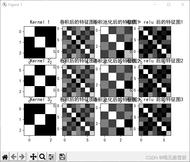
3. 可视化:了解数字与图像之间的关系
可视化卷积核与特征图
import torch
import torch.nn as nn
import matplotlib.pyplot as plt
plt.rcParams['font.sans-serif'] = ['SimHei'] # 用来正常显示中文标签
plt.rcParams['axes.unicode_minus'] = False # 用来正常显示负号 #有中文出现的情况,需要u'内容
x = torch.tensor([[[[-1, -1, -1, -1, -1, -1, -1, -1, -1],
[-1, 1, -1, -1, -1, -1, -1, 1, -1],
[-1, -1, 1, -1, -1, -1, 1, -1, -1],
[-1, -1, -1, 1, -1, 1, -1, -1, -1],
[-1, -1, -1, -1, 1, -1, -1, -1, -1],
[-1, -1, -1, 1, -1, 1, -1, -1, -1],
[-1, -1, 1, -1, -1, -1, 1, -1, -1],
[-1, 1, -1, -1, -1, -1, -1, 1, -1],
[-1, -1, -1, -1, -1, -1, -1, -1, -1]]]], dtype=torch.float)
print(x.shape)
print(x)
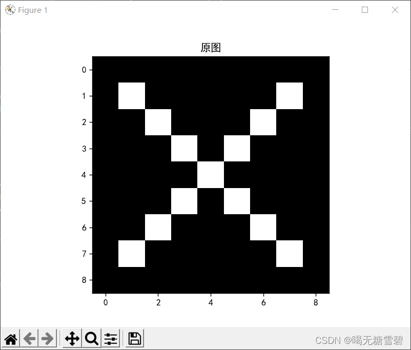
img = x.data.squeeze().numpy() # 将输出转换为图片的格式
plt.imshow(img, cmap='gray')
plt.title('原图')
plt.show()
print("--------------- 卷积 ---------------")
conv1 = nn.Conv2d(1, 1, (3, 3), 1) # in_channel , out_channel , kennel_size , stride
conv1.weight.data = torch.Tensor([[[[1, -1, -1],
[-1, 1, -1],
[-1, -1, 1]]
]])
img = conv1.weight.data.squeeze().numpy() # 将输出转换为图片的格式
plt.subplot(3, 4, 1)
plt.imshow(img, cmap='gray')
plt.title('Kernel 1')
conv2 = nn.Conv2d(1, 1, (3, 3), 1) # in_channel , out_channel , kennel_size , stride
conv2.weight.data = torch.Tensor([[[[1, -1, 1],
[-1, 1, -1],
[1, -1, 1]]
]])
img = conv2.weight.data.squeeze().numpy() # 将输出转换为图片的格式
plt.subplot(3, 4, 5)
plt.imshow(img, cmap='gray')
plt.title('Kernel 2')
conv3 = nn.Conv2d(1, 1, (3, 3), 1) # in_channel , out_channel , kennel_size , stride
conv3.weight.data = torch.Tensor([[[[-1, -1, 1],
[-1, 1, -1],
[1, -1, -1]]
]])
img = conv3.weight.data.squeeze().numpy() # 将输出转换为图片的格式
plt.subplot(3, 4, 9)
plt.imshow(img, cmap='gray')
plt.title('Kernel 3')
feature_map1 = conv1(x)
feature_map2 = conv2(x)
feature_map3 = conv3(x)
print(feature_map1 / 9)
print(feature_map2 / 9)
print(feature_map3 / 9)
img = feature_map1.data.squeeze().numpy() # 将输出转换为图片的格式
plt.subplot(3, 4, 2)
plt.imshow(img, cmap='gray')
plt.title('卷积后的特征图1')
img2 = feature_map2.data.squeeze().numpy() # 将输出转换为图片的格式
plt.subplot(3, 4, 6)
plt.imshow(img, cmap='gray')
plt.title('卷积后的特征图2')
img3 = feature_map3.data.squeeze().numpy() # 将输出转换为图片的格式
plt.subplot(3, 4, 10)
plt.imshow(img, cmap='gray')
plt.title('卷积后的特征图3')
print("--------------- 池化 ---------------")
max_pool = nn.MaxPool2d(2, padding=0, stride=2) # Pooling
zeroPad = nn.ZeroPad2d(padding=(0, 1, 0, 1)) # pad 0 , Left Right Up Down
feature_map_pad_0_1 = zeroPad(feature_map1)
feature_pool_1 = max_pool(feature_map_pad_0_1)
feature_map_pad_0_2 = zeroPad(feature_map2)
feature_pool_2 = max_pool(feature_map_pad_0_2)
feature_map_pad_0_3 = zeroPad(feature_map3)
feature_pool_3 = max_pool(feature_map_pad_0_3)
print(feature_pool_1.size())
print(feature_pool_1 / 9)
print(feature_pool_2 / 9)
print(feature_pool_3 / 9)
img = feature_pool_1.data.squeeze().numpy() # 将输出转换为图片的格式
plt.subplot(3, 4, 3)
plt.imshow(img, cmap='gray')
plt.title('卷积池化后的特征图1')
img2 = feature_pool_2.data.squeeze().numpy() # 将输出转换为图片的格式
plt.subplot(3, 4, 7)
plt.imshow(img, cmap='gray')
plt.title('卷积池化后的特征图2')
img3 = feature_pool_3.data.squeeze().numpy() # 将输出转换为图片的格式
plt.subplot(3, 4, 11)
plt.imshow(img, cmap='gray')
plt.title('卷积池化后的特征图3')
print("--------------- 激活 ---------------")
activation_function = nn.ReLU()
feature_relu1 = activation_function(feature_map1)
feature_relu2 = activation_function(feature_map2)
feature_relu3 = activation_function(feature_map3)
print(feature_relu1 / 9)
print(feature_relu2 / 9)
print(feature_relu3 / 9)
img = feature_relu1.data.squeeze().numpy() # 将输出转换为图片的格式
plt.subplot(3, 4, 4)
plt.imshow(img, cmap='gray')
plt.title('卷积 + relu 后的特征图1')
img2 = feature_relu2.data.squeeze().numpy() # 将输出转换为图片的格式
plt.subplot(3, 4, 8)
plt.imshow(img, cmap='gray')
plt.title('卷积 + relu 后的特征图2')
img3 = feature_relu3.data.squeeze().numpy() # 将输出转换为图片的格式
plt.subplot(3, 4, 12)
plt.imshow(img, cmap='gray')
plt.title('卷积 + relu 后的特征图3')
plt.show()运行结果:
torch.Size([1, 1, 9, 9])
tensor([[[[-1., -1., -1., -1., -1., -1., -1., -1., -1.],
          [-1.,  1., -1., -1., -1., -1., -1.,  1., -1.],
          [-1., -1.,  1., -1., -1., -1.,  1., -1., -1.],
          [-1., -1., -1.,  1., -1.,  1., -1., -1., -1.],
          [-1., -1., -1., -1.,  1., -1., -1., -1., -1.],
          [-1., -1., -1.,  1., -1.,  1., -1., -1., -1.],
          [-1., -1.,  1., -1., -1., -1.,  1., -1., -1.],
          [-1.,  1., -1., -1., -1., -1., -1.,  1., -1.],
          [-1., -1., -1., -1., -1., -1., -1., -1., -1.]]]])
--------------- 卷积  ---------------
tensor([[[[ 0.7540, -0.1349,  0.0873,  0.3095,  0.5318, -0.1349,  0.3095],
          [-0.1349,  0.9762, -0.1349,  0.3095, -0.1349,  0.0873, -0.1349],
          [ 0.0873, -0.1349,  0.9762, -0.3571,  0.0873, -0.1349,  0.5318],
          [ 0.3095,  0.3095, -0.3571,  0.5318, -0.3571,  0.3095,  0.3095],
          [ 0.5318, -0.1349,  0.0873, -0.3571,  0.9762, -0.1349,  0.0873],
          [-0.1349,  0.0873, -0.1349,  0.3095, -0.1349,  0.9762, -0.1349],
          [ 0.3095, -0.1349,  0.5318,  0.3095,  0.0873, -0.1349,  0.7540]]]],
       grad_fn=<DivBackward0>)
tensor([[[[ 0.3604, -0.5285,  0.1382, -0.0840,  0.1382, -0.5285,  0.3604],
          [-0.5285,  0.5826, -0.5285,  0.3604, -0.5285,  0.5826, -0.5285],
          [ 0.1382, -0.5285,  0.5826, -0.7507,  0.5826, -0.5285,  0.1382],
          [-0.0840,  0.3604, -0.7507,  1.0271, -0.7507,  0.3604, -0.0840],
          [ 0.1382, -0.5285,  0.5826, -0.7507,  0.5826, -0.5285,  0.1382],
          [-0.5285,  0.5826, -0.5285,  0.3604, -0.5285,  0.5826, -0.5285],
          [ 0.3604, -0.5285,  0.1382, -0.0840,  0.1382, -0.5285,  0.3604]]]],
       grad_fn=<DivBackward0>)
tensor([[[[ 0.3072, -0.1372,  0.5294,  0.3072,  0.0850, -0.1372,  0.7517],
          [-0.1372,  0.0850, -0.1372,  0.3072, -0.1372,  0.9739, -0.1372],
          [ 0.5294, -0.1372,  0.0850, -0.3594,  0.9739, -0.1372,  0.0850],
          [ 0.3072,  0.3072, -0.3594,  0.5294, -0.3594,  0.3072,  0.3072],
          [ 0.0850, -0.1372,  0.9739, -0.3594,  0.0850, -0.1372,  0.5294],
          [-0.1372,  0.9739, -0.1372,  0.3072, -0.1372,  0.0850, -0.1372],
          [ 0.7517, -0.1372,  0.0850,  0.3072,  0.5294, -0.1372,  0.3072]]]],
       grad_fn=<DivBackward0>)
--------------- 池化  ---------------
torch.Size([1, 1, 4, 4])
tensor([[[[0.9762, 0.3095, 0.5318, 0.3095],
          [0.3095, 0.9762, 0.3095, 0.5318],
          [0.5318, 0.3095, 0.9762, 0.0873],
          [0.3095, 0.5318, 0.0873, 0.7540]]]], grad_fn=<DivBackward0>)
tensor([[[[0.5826, 0.3604, 0.5826, 0.3604],
          [0.3604, 1.0271, 0.5826, 0.1382],
          [0.5826, 0.5826, 0.5826, 0.1382],
          [0.3604, 0.1382, 0.1382, 0.3604]]]], grad_fn=<DivBackward0>)
tensor([[[[0.3072, 0.5294, 0.9739, 0.7517],
          [0.5294, 0.5294, 0.9739, 0.3072],
          [0.9739, 0.9739, 0.0850, 0.5294],
          [0.7517, 0.3072, 0.5294, 0.3072]]]], grad_fn=<DivBackward0>)
--------------- 激活  ---------------
tensor([[[[0.7540, 0.0000, 0.0873, 0.3095, 0.5318, 0.0000, 0.3095],
          [0.0000, 0.9762, 0.0000, 0.3095, 0.0000, 0.0873, 0.0000],
          [0.0873, 0.0000, 0.9762, 0.0000, 0.0873, 0.0000, 0.5318],
          [0.3095, 0.3095, 0.0000, 0.5318, 0.0000, 0.3095, 0.3095],
          [0.5318, 0.0000, 0.0873, 0.0000, 0.9762, 0.0000, 0.0873],
          [0.0000, 0.0873, 0.0000, 0.3095, 0.0000, 0.9762, 0.0000],
          [0.3095, 0.0000, 0.5318, 0.3095, 0.0873, 0.0000, 0.7540]]]],
       grad_fn=<DivBackward0>)
tensor([[[[0.3604, 0.0000, 0.1382, 0.0000, 0.1382, 0.0000, 0.3604],
          [0.0000, 0.5826, 0.0000, 0.3604, 0.0000, 0.5826, 0.0000],
          [0.1382, 0.0000, 0.5826, 0.0000, 0.5826, 0.0000, 0.1382],
          [0.0000, 0.3604, 0.0000, 1.0271, 0.0000, 0.3604, 0.0000],
          [0.1382, 0.0000, 0.5826, 0.0000, 0.5826, 0.0000, 0.1382],
          [0.0000, 0.5826, 0.0000, 0.3604, 0.0000, 0.5826, 0.0000],
          [0.3604, 0.0000, 0.1382, 0.0000, 0.1382, 0.0000, 0.3604]]]],
       grad_fn=<DivBackward0>)
tensor([[[[0.3072, 0.0000, 0.5294, 0.3072, 0.0850, 0.0000, 0.7517],
          [0.0000, 0.0850, 0.0000, 0.3072, 0.0000, 0.9739, 0.0000],
          [0.5294, 0.0000, 0.0850, 0.0000, 0.9739, 0.0000, 0.0850],
          [0.3072, 0.3072, 0.0000, 0.5294, 0.0000, 0.3072, 0.3072],
          [0.0850, 0.0000, 0.9739, 0.0000, 0.0850, 0.0000, 0.5294],
          [0.0000, 0.9739, 0.0000, 0.3072, 0.0000, 0.0850, 0.0000],
          [0.7517, 0.0000, 0.0850, 0.3072, 0.5294, 0.0000, 0.3072]]]],
       grad_fn=<DivBackward0>)
二、 基于CNN的XO识别
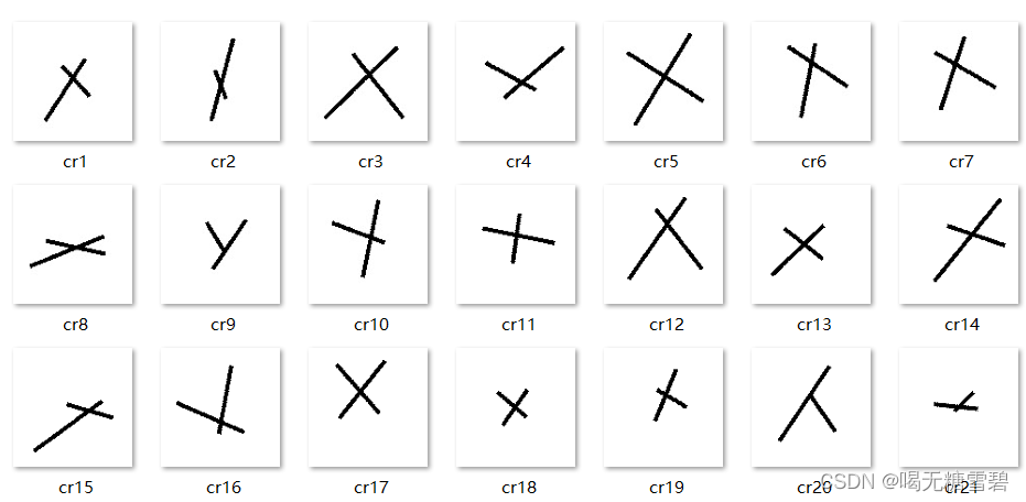
1. 数据集
共2000张图片,X、O各1000张。
从X、O文件夹,分别取出150张作为测试集。
文件夹train_data:放置训练集 1700张图片
文件夹test_data: 放置测试集 300张图片
部分数据如下: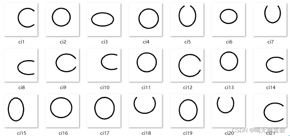
2. 构建模型
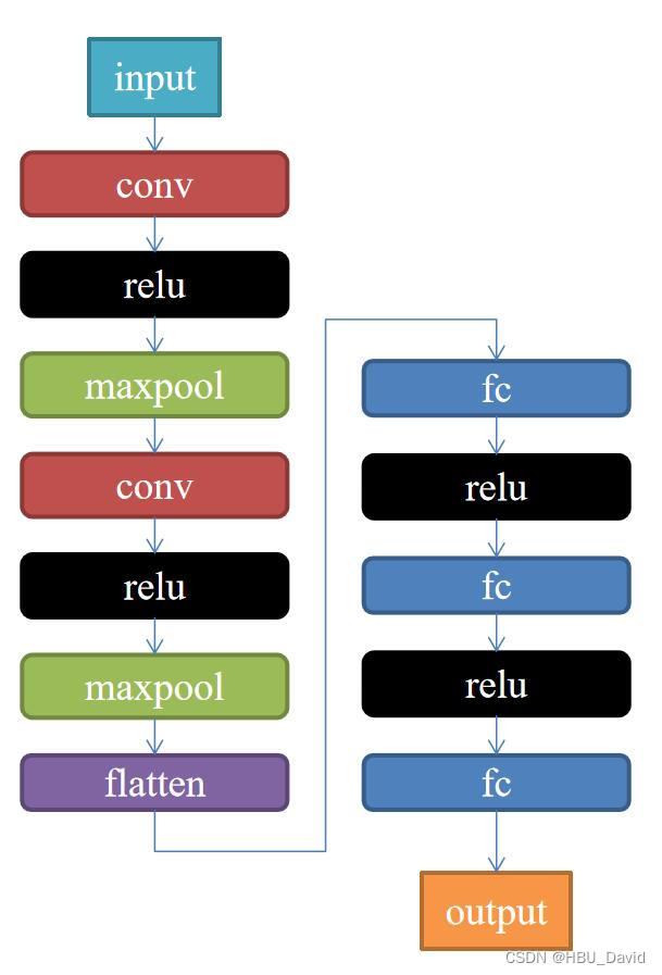
代码如下:
import torch
import torch.nn as nn


#构建模型
class Net(nn.Module):
    def __init__(self):
        super(Net, self).__init__()
        self.conv1 = nn.Conv2d(1, 9, 3)
        self.maxpool = nn.MaxPool2d(2, 2)
        self.conv2 = nn.Conv2d(9, 5, 3)

        self.relu = nn.ReLU()
        self.fc1 = nn.Linear(27 * 27 * 5, 1200)
        self.fc2 = nn.Linear(1200, 64)
        self.fc3 = nn.Linear(64, 2)

    def forward(self, x):
        x = self.maxpool(self.relu(self.conv1(x)))
        x = self.maxpool(self.relu(self.conv2(x)))
        x = x.view(-1, 27 * 27 * 5)
        x = self.relu(self.fc1(x))
        x = self.relu(self.fc2(x))
        x = self.fc3(x)
        return x
3. 训练模型
代码实现:
#训练模型
import torch
from torchvision import transforms, datasets
import torch.nn as nn
from torch.utils.data import DataLoader
import matplotlib.pyplot as plt
import torch.optim as optim
transforms = transforms.Compose([
transforms.ToTensor(), # 把图片进行归一化,并把数据转换成Tensor类型
transforms.Grayscale(1) # 把图片 转为灰度图
])
path = r'train_data'
path_test = r'test_data'
data_train = datasets.ImageFolder(path, transform=transforms)
data_test = datasets.ImageFolder(path_test, transform=transforms)
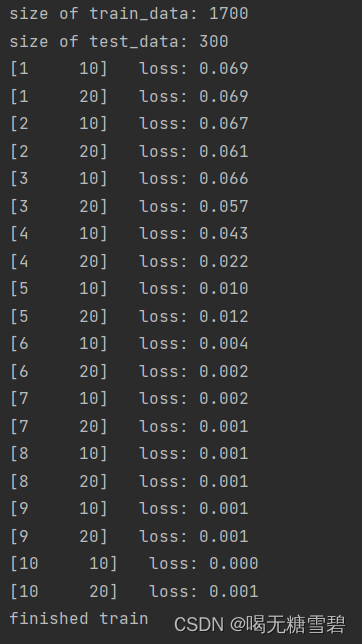
print("size of train_data:", len(data_train))
print("size of test_data:", len(data_test))
data_loader = DataLoader(data_train, batch_size=64, shuffle=True)
data_loader_test = DataLoader(data_test, batch_size=64, shuffle=True)
model = Net()
criterion = torch.nn.CrossEntropyLoss() # 损失函数 交叉熵损失函数
optimizer = optim.SGD(model.parameters(), lr=0.1) # 优化函数:随机梯度下降
epochs = 10
for epoch in range(epochs):
running_loss = 0.0
for i, data in enumerate(data_loader):
images, label = data
out = model(images)
loss = criterion(out, label)
optimizer.zero_grad()
loss.backward()
optimizer.step()
running_loss += loss.item()
if (i + 1) % 10 == 0:
print('[%d %5d] loss: %.3f' % (epoch + 1, i + 1, running_loss / 100))
running_loss = 0.0
print('finished train')运行结果
4. 测试训练好的模型
代码实现:
# 保存模型
torch.save(model, 'model_name.pth') # 保存的是模型, 不止是w和b权重值
#测试训练好的模型
# 读取模型
model_load = torch.load('model_name.pth')
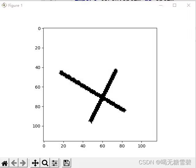
# 读取一张图片 images[0],测试
print("label[0] truth:\t", label[0])
x = images[0]
predicted = torch.max(model_load(x), 1)
print("label[0] predict:\t", predicted.indices)
img = images[0].data.squeeze().numpy() # 将输出转换为图片的格式
plt.imshow(img, cmap='gray')
plt.show()运行结果:
5. 计算模型的准确率
# 读取模型
model_load = Net()
model_load = torch.load('model_name.pth')
correct = 0
total = 0
with torch.no_grad():  # 进行评测的时候网络不更新梯度
    for data in data_loader_test:  # 读取测试集
        images, labels = data
        outputs = model_load(images)
        _, predicted = torch.max(outputs.data, 1)  # 取出 最大值的索引 作为 分类结果
        total += labels.size(0)  # labels 的长度
        correct += (predicted == labels).sum().item()  # 预测正确的数目
print('Accuracy of the network on the  test images: %f %%' % (100. * correct / total))
运行结果:
![]()
6. 查看训练好的模型的特征图
# 看看每层的 卷积核 长相,特征图 长相
# 获取网络结构的特征矩阵并可视化
import torch
import matplotlib.pyplot as plt
import numpy as np
from PIL import Image
from torchvision import transforms, datasets
import torch.nn as nn
from torch.utils.data import DataLoader
# 定义图像预处理过程(要与网络模型训练过程中的预处理过程一致)
transforms = transforms.Compose([
transforms.ToTensor(), # 把图片进行归一化,并把数据转换成Tensor类型
transforms.Grayscale(1) # 把图片 转为灰度图
])
path = r'train_data'
data_train = datasets.ImageFolder(path, transform=transforms)
data_loader = DataLoader(data_train, batch_size=64, shuffle=True)
for i, data in enumerate(data_loader):
images, labels = data
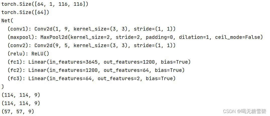
print(images.shape)
print(labels.shape)
break
class Net(nn.Module):
def __init__(self):
super(Net, self).__init__()
self.conv1 = nn.Conv2d(1, 9, 3) # in_channel , out_channel , kennel_size , stride
self.maxpool = nn.MaxPool2d(2, 2)
self.conv2 = nn.Conv2d(9, 5, 3) # in_channel , out_channel , kennel_size , stride
self.relu = nn.ReLU()
self.fc1 = nn.Linear(27 * 27 * 5, 1200) # full connect 1
self.fc2 = nn.Linear(1200, 64) # full connect 2
self.fc3 = nn.Linear(64, 2) # full connect 3
def forward(self, x):
outputs = []
x = self.conv1(x)
outputs.append(x)
x = self.relu(x)
outputs.append(x)
x = self.maxpool(x)
outputs.append(x)
x = self.conv2(x)
x = self.relu(x)
x = self.maxpool(x)
x = x.view(-1, 27 * 27 * 5)
x = self.relu(self.fc1(x))
x = self.relu(self.fc2(x))
x = self.fc3(x)
return outputs
# create model
model1 = Net()
# load model weights加载预训练权重
# model_weight_path ="./AlexNet.pth"
model_weight_path = "model_name.pth"
model1 = torch.load(model_weight_path)
# 打印出模型的结构
print(model1)
x = images[0]
x = x.reshape([1, 1, 116, 116])
# forward正向传播过程
out_put = model1(x)
for feature_map in out_put:
# [N, C, H, W] -> [C, H, W] 维度变换
im = np.squeeze(feature_map.detach().numpy())
# [C, H, W] -> [H, W, C]
im = np.transpose(im, [1, 2, 0])
print(im.shape)
# show 9 feature maps
plt.figure()
for i in range(9):
ax = plt.subplot(3, 3, i + 1) # 参数意义:3:图片绘制行数,5:绘制图片列数,i+1:图的索引
# [H, W, C]
# 特征矩阵每一个channel对应的是一个二维的特征矩阵,就像灰度图像一样,channel=1
# plt.imshow(im[:, :, i])
plt.imshow(im[:, :, i], cmap='gray')
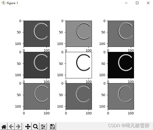
plt.show()运行结果
第一轮卷积后的图像
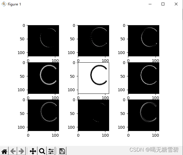
第二轮卷积后二图像
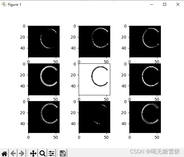
第三轮卷积后的图像
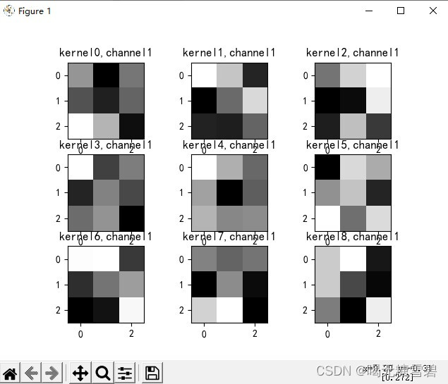
7. 查看训练好的模型的卷积核
#查看训练好的卷积核
# 看看每层的 卷积核 长相,特征图 长相
# 获取网络结构的特征矩阵并可视化
import torch
import matplotlib.pyplot as plt
import numpy as np
from PIL import Image
from torchvision import transforms, datasets
import torch.nn as nn
from torch.utils.data import DataLoader

plt.rcParams['font.sans-serif'] = ['SimHei']  # 用来正常显示中文标签
plt.rcParams['axes.unicode_minus'] = False  # 用来正常显示负号 #有中文出现的情况,需要u'内容
#  定义图像预处理过程(要与网络模型训练过程中的预处理过程一致)
transforms = transforms.Compose([
    transforms.ToTensor(),  # 把图片进行归一化,并把数据转换成Tensor类型
    transforms.Grayscale(1)  # 把图片 转为灰度图
])
path = r'train_data'
data_train = datasets.ImageFolder(path, transform=transforms)
data_loader = DataLoader(data_train, batch_size=64, shuffle=True)
for i, data in enumerate(data_loader):
    images, labels = data
    # print(images.shape)
    # print(labels.shape)
    break


class Net(nn.Module):
    def __init__(self):
        super(Net, self).__init__()
        self.conv1 = nn.Conv2d(1, 9, 3)  # in_channel , out_channel , kennel_size , stride
        self.maxpool = nn.MaxPool2d(2, 2)
        self.conv2 = nn.Conv2d(9, 5, 3)  # in_channel , out_channel , kennel_size , stride

        self.relu = nn.ReLU()
        self.fc1 = nn.Linear(27 * 27 * 5, 1200)  # full connect 1
        self.fc2 = nn.Linear(1200, 64)  # full connect 2
        self.fc3 = nn.Linear(64, 2)  # full connect 3

    def forward(self, x):
        outputs = []
        x = self.maxpool(self.relu(self.conv1(x)))
        # outputs.append(x)
        x = self.maxpool(self.relu(self.conv2(x)))
        outputs.append(x)
        x = x.view(-1, 27 * 27 * 5)
        x = self.relu(self.fc1(x))
        x = self.relu(self.fc2(x))
        x = self.fc3(x)
        return outputs


# create model
model1 = Net()

# load model weights加载预训练权重
model_weight_path = "model_name.pth"
model1 = torch.load(model_weight_path)

x = images[0]
x = x.reshape([1, 1, 116, 116])
# forward正向传播过程
out_put = model1(x)

weights_keys = model1.state_dict().keys()
for key in weights_keys:
    print("key :", key)
    # 卷积核通道排列顺序 [kernel_number, kernel_channel, kernel_height, kernel_width]
    if key == "conv1.weight":
        weight_t = model1.state_dict()[key].numpy()
        print("weight_t.shape", weight_t.shape)
        k = weight_t[:, 0, :, :]  # 获取第一个卷积核的信息参数
        # show 9 kernel ,1 channel
        plt.figure()

        for i in range(9):
            ax = plt.subplot(3, 3, i + 1)  # 参数意义:3:图片绘制行数,5:绘制图片列数,i+1:图的索引
            plt.imshow(k[i, :, :], cmap='gray')
            title_name = 'kernel' + str(i) + ',channel1'
            plt.title(title_name)
        plt.show()

    if key == "conv2.weight":
        weight_t = model1.state_dict()[key].numpy()
        print("weight_t.shape", weight_t.shape)
        k = weight_t[:, :, :, :]  # 获取第一个卷积核的信息参数
        print(k.shape)
        print(k)

        plt.figure()
        for c in range(9):
            channel = k[:, c, :, :]
            for i in range(5):
                ax = plt.subplot(2, 3, i + 1)  # 参数意义:3:图片绘制行数,5:绘制图片列数,i+1:图的索引
                plt.imshow(channel[i, :, :], cmap='gray')
                title_name = 'kernel' + str(i) + ',channel' + str(c)
                plt.title(title_name)
            plt.show()
运行结果:
8. 训练模型源代码
# https://blog.csdn.net/qq_53345829/article/details/124308515
import torch
from torchvision import transforms, datasets
import torch.nn as nn
from torch.utils.data import DataLoader
import matplotlib.pyplot as plt
import torch.optim as optim

transforms = transforms.Compose([
    transforms.ToTensor(),  # 把图片进行归一化,并把数据转换成Tensor类型
    transforms.Grayscale(1)  # 把图片 转为灰度图
])

path = r'C:\Users\ASUS\Desktop\深度学习\training_data_sm\train_data'
path_test = r'C:\Users\ASUS\Desktop\深度学习\training_data_sm\train_data'

data_train = datasets.ImageFolder(path, transform=transforms)
data_test = datasets.ImageFolder(path_test, transform=transforms)

print("size of train_data:", len(data_train))
print("size of test_data:", len(data_test))

data_loader = DataLoader(data_train, batch_size=64, shuffle=True)
data_loader_test = DataLoader(data_test, batch_size=64, shuffle=True)

for i, data in enumerate(data_loader):
    images, labels = data
    print(images.shape)
    print(labels.shape)
    break

for i, data in enumerate(data_loader_test):
    images, labels = data
    print(images.shape)
    print(labels.shape)
    break


class Net(nn.Module):
    def __init__(self):
        super(Net, self).__init__()
        self.conv1 = nn.Conv2d(1, 9, 3)  # in_channel , out_channel , kennel_size , stride
        self.maxpool = nn.MaxPool2d(2, 2)
        self.conv2 = nn.Conv2d(9, 5, 3)  # in_channel , out_channel , kennel_size , stride

        self.relu = nn.ReLU()
        self.fc1 = nn.Linear(27 * 27 * 5, 1200)  # full connect 1
        self.fc2 = nn.Linear(1200, 64)  # full connect 2
        self.fc3 = nn.Linear(64, 2)  # full connect 3

    def forward(self, x):
        x = self.maxpool(self.relu(self.conv1(x)))
        x = self.maxpool(self.relu(self.conv2(x)))
        x = x.view(-1, 27 * 27 * 5)
        x = self.relu(self.fc1(x))
        x = self.relu(self.fc2(x))
        x = self.fc3(x)
        return x


model = Net()

criterion = torch.nn.CrossEntropyLoss()  # 损失函数 交叉熵损失函数
optimizer = optim.SGD(model.parameters(), lr=0.1)  # 优化函数:随机梯度下降

epochs = 10
for epoch in range(epochs):
    running_loss = 0.0
    for i, data in enumerate(data_loader):
        images, label = data
        out = model(images)
        loss = criterion(out, label)

        optimizer.zero_grad()
        loss.backward()
        optimizer.step()

        running_loss += loss.item()
        if (i + 1) % 10 == 0:
            print('[%d  %5d]   loss: %.3f' % (epoch + 1, i + 1, running_loss / 100))
            running_loss = 0.0

print('finished train')

# 保存模型 torch.save(model.state_dict(), model_path)
torch.save(model.state_dict(), 'model_name1.pth')  # 保存的是模型, 不止是w和b权重值

# 读取模型
model = torch.load('model_name1.pth')
9. 测试模型源代码
import torch
from torchvision import transforms, datasets
import torch.nn as nn
from torch.utils.data import DataLoader
import matplotlib.pyplot as plt
import torch.optim as optim

transforms = transforms.Compose([
    transforms.ToTensor(),  # 把图片进行归一化,并把数据转换成Tensor类型
    transforms.Grayscale(1)  # 把图片 转为灰度图
])

path = r'train_data'
path_test = r'train_data'

data_train = datasets.ImageFolder(path, transform=transforms)
data_test = datasets.ImageFolder(path_test, transform=transforms)

print("size of train_data:", len(data_train))
print("size of test_data:", len(data_test))

data_loader = DataLoader(data_train, batch_size=64, shuffle=True)
data_loader_test = DataLoader(data_test, batch_size=64, shuffle=True)
print(len(data_loader))
print(len(data_loader_test))


class Net(nn.Module):
    def __init__(self):
        super(Net, self).__init__()
        self.conv1 = nn.Conv2d(1, 9, 3)  # in_channel , out_channel , kennel_size , stride
        self.maxpool = nn.MaxPool2d(2, 2)
        self.conv2 = nn.Conv2d(9, 5, 3)  # in_channel , out_channel , kennel_size , stride

        self.relu = nn.ReLU()
        self.fc1 = nn.Linear(27 * 27 * 5, 1200)  # full connect 1
        self.fc2 = nn.Linear(1200, 64)  # full connect 2
        self.fc3 = nn.Linear(64, 2)  # full connect 3

    def forward(self, x):
        x = self.maxpool(self.relu(self.conv1(x)))
        x = self.maxpool(self.relu(self.conv2(x)))
        x = x.view(-1, 27 * 27 * 5)
        x = self.relu(self.fc1(x))
        x = self.relu(self.fc2(x))
        x = self.fc3(x)
        return x


# 读取模型
model = Net()
model.load_state_dict(torch.load('model_name1.pth', map_location='cpu'))  # 导入网络的参数

# model_load = torch.load('model_name1.pth')
# https://blog.csdn.net/qq_41360787/article/details/104332706

correct = 0
total = 0
with torch.no_grad():  # 进行评测的时候网络不更新梯度
    for data in data_loader_test:  # 读取测试集
        images, labels = data
        outputs = model(images)
        _, predicted = torch.max(outputs.data, 1)  # 取出 最大值的索引 作为 分类结果
        total += labels.size(0)  # labels 的长度
        correct += (predicted == labels).sum().item()  # 预测正确的数目
print('Accuracy of the network on the  test images: %f %%' % (100. * correct / total))

#  "_," 的解释 https://blog.csdn.net/weixin_48249563/article/details/111387501


 7848
7848


 被折叠的 条评论
为什么被折叠?
被折叠的 条评论
为什么被折叠?
 到【灌水乐园】发言


