


1. Logistic Regression
1.1 Visualizing the data
Data:学生两次测试的分数、是否被录取(0/1表示)
plot.py
import matplotlib.pyplot as plt  # 数据图形化

def Plot(data):
    # isin函数接收列表
    positive = data[data.Admitted.isin([1])]  # 正样本
    negative = data[data.Admitted.isin([0])]  # 负样本

    # 绘图
    # fig:代表绘图窗口(Figure)
    # ax:绘图窗口上的坐标系(axis),一般会对它继续操作

    # 下面两行代码可简写成:fig, ax = plt.subplots(figsize=(12, 8))
    # 注意subplots()既创建了一个包含子图区域的画布,又创建了一个figure图形对象,
    # 而subplot()只是创建一个包含子图区域的画布
    fig = plt.figure(figsize=(10, 6))
    ax = fig.add_subplot(1, 1, 1)  # subplots(a,b,c):a-子图行、b-子图列数、c-第c个子图
    # c-color、s-area
    ax.scatter(positive['Exam1'], positive['Exam2'], c='b', s=50, marker='o', label='Admitted')
    ax.scatter(negative['Exam1'], negative['Exam2'], c='r', s=50, marker='x', label='Not Admitted')
    ax.legend()  # 图例说明
    ax.set_xlabel('Exam1 Score')
    ax.set_ylabel('Exam2 Score')
    plt.show()
main.py
import pandas as pd  # 一种用于数据分析的扩展程序库
import plot as pl

data = pd.read_csv(
    'ex2data1.txt',
    header=None,
    names=['Exam1', 'Exam2', 'Admitted']
)
pl.Plot(data)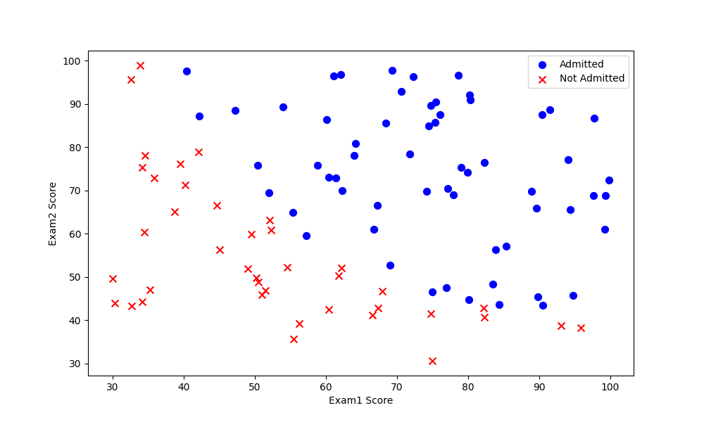
1.2 Implementation
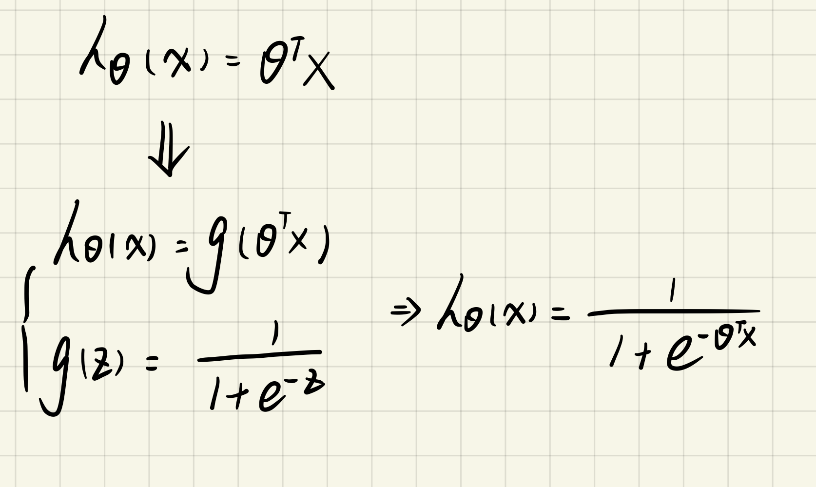
1.2.1 sigmoid function
sigmoid.py
import numpy as np  # 矩阵

def Sigmoid(z):
    return 1 / (1 + np.exp(-z))
1.2.2 Cost function and gradient

costFunction.py
import numpy as np
from sigmoid import *  # sigmoid函数

def costFunction(theta, X, y):
    X = np.matrix(X)
    y = np.matrix(y)
    theta = np.matrix(theta)
    # multiply:对应位置相乘,*:矩阵乘法
    c1 = np.multiply(y, np.log(Sigmoid(X * theta.T)))
    c2 = np.multiply(1 - y, np.log(1 - Sigmoid(X * theta.T)))
    return -(1 / len(X)) * np.sum(c1 + c2)
main.py
import pandas as pd  # 一种用于数据分析的扩展程序库
import numpy as np  # 矩阵
import plot as pl  # 绘图
from costFunction import *  # 代价函数

data = pd.read_csv(
    'ex2data1.txt',
    header=None,
    names=['Exam1', 'Exam2', 'Admitted']
)
# pl.Plot(data)

# 初始化数据
data.insert(0, 'Zeros', 1)
cols = data.shape[1]
X = data.iloc[:, 0:cols - 1].values
y = data.iloc[:, cols - 1:cols].values
theta = np.zeros(X.shape[1])
print(costFunction(theta, X, y))  # 0.6931471805599453

# 梯度下降
alpha = 0.01
iteration = 1000
theta = gradientDescent(theta, X, y, alpha, iteration)
gradientDescent.py
import numpy as np  # 矩阵
from sigmoid import *  # sigmoid函数
from costFunction import *  # 代价函数


def gradientDescent(theta, X, y, alpha, iteration):
    X = np.matrix(X)
    y = np.matrix(y)
    theta = np.matrix(theta)
    para_theta_num = theta.shape[1]
    theta_temp = np.matrix(np.zeros(para_theta_num))

    for i in range(iteration):
        theta_temp = theta - (alpha / len(X)) * ((Sigmoid(X * theta.T) - y).T * X)
        theta = theta_temp
    return theta
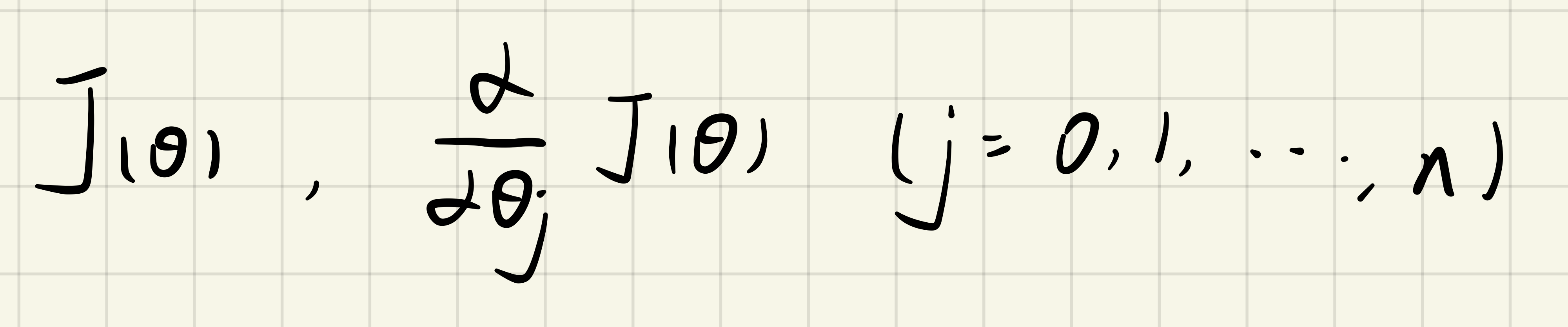
1.2.3 Advanced Optimization
gradientDescent.py
修改:求对代价函数J(theta)的导数,不需要有alpha和iters
import numpy as np  # 矩阵
from sigmoid import *  # sigmoid函数


def gradientDescent(theta, X, y):
    X = np.matrix(X)
    y = np.matrix(y)
    theta = np.matrix(theta)
    para_theta_num = theta.shape[1]
    grad = np.zeros(para_theta_num)
    for i in range(para_theta_num):
        # 代价函数的导数
        grad[i] = ((Sigmoid(X * theta.T) - y).T * X[:, i]) / len(X)
return grad注意:theta作为costFunction和gradientDescent函数的参数时要放在最前面
main.py
import pandas as pd  # 一种用于数据分析的扩展程序库
import numpy as np  # 矩阵
import plot as pl  # 绘图
from costFunction import *  # 代价函数
from gradientDescent import *  # 梯度下降
import scipy.optimize as opt  # scipy优化算法

data = pd.read_csv(
    'ex2data1.txt',
    header=None,
    names=['Exam1', 'Exam2', 'Admitted']
)
# pl.Plot(data)

# 初始化数据
data.insert(0, 'Zeros', 1)
cols = data.shape[1]
X = data.iloc[:, 0:cols - 1].values
y = data.iloc[:, cols - 1:cols].values
theta = np.zeros(X.shape[1])

# 参数
# func: 优化的目标函数
# x0: 初值
# fprime: 提供优化函数func的梯度函数
# args: 传递给优化函数的参数
#
# 返回值
# x: 优化函数的目标值

result = opt.fmin_tnc(func=costFunction, x0=theta, fprime=gradientDescent, args=(X, y))
print(result)
print(costFunction(result[0], X, y))

# (array([-25.16131857,   0.20623159,   0.20147149]), 36, 0)
# 0.20349770158947486
1.2.4 Plot The Decision Boundary
main.py
import pandas as pd # 一种用于数据分析的扩展程序库
import numpy as np # 矩阵
import matplotlib.pyplot as plt # 数据图形化
from costFunction import * # 代价函数
from gradientDescent import * # 梯度下降
import scipy.optimize as opt # scipy优化算法
data = pd.read_csv(
'ex2data1.txt',
header=None,
names=['Exam1', 'Exam2', 'Admitted']
)
# 初始化数据
data.insert(0, 'Zeros', 1)
cols = data.shape[1]
X = data.iloc[:, 0:cols - 1].values
y = data.iloc[:, cols - 1:cols].values
theta = np.zeros(X.shape[1])
result = opt.fmin_tnc(func=costFunction, x0=theta, fprime=gradientDescent, args=(X, y))
theta = result[0] # 最优theta
positive = data[data.Admitted.isin([1])] # 正样本
negative = data[data.Admitted.isin([0])] # 负样本
fig = plt.figure(figsize=(10, 6))
ax = fig.add_subplot(1, 1, 1)
ax.scatter(positive['Exam1'], positive['Exam2'], c='b', s=50, marker='o', label='Admitted')
ax.scatter(negative['Exam1'], negative['Exam2'], c='r', s=50, marker='x', label='Not Admitted')
ax.set_xlabel('Exam1 Score')
ax.set_ylabel('Exam2 Score')
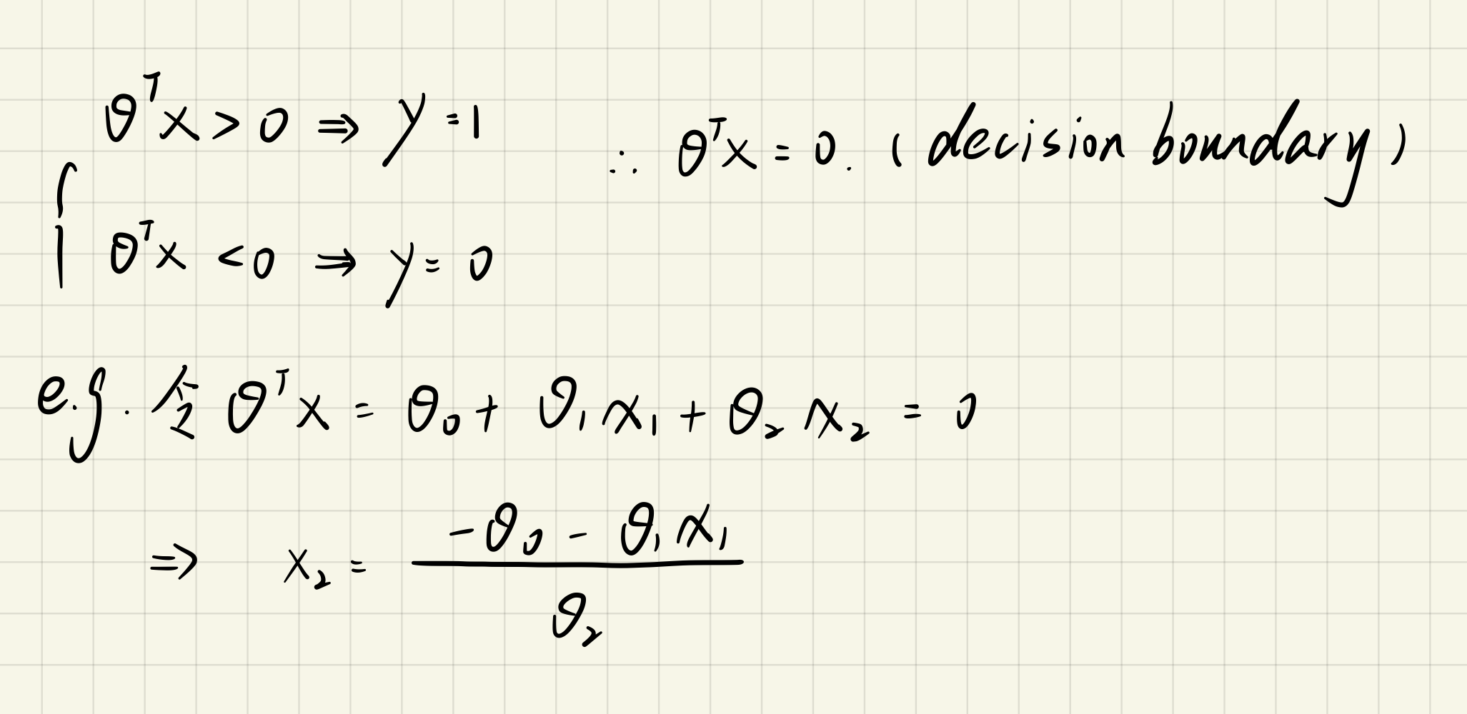
x1 = np.linspace(30, 100, 100)
h1 = (-theta[0] - theta[1] * x1) / theta[2]
ax.plot(x1, h1, 'g', label='Prediction') # g:green
ax.legend() # 图例说明
plt.show()

1.2.5 Evaluate logistic regression
predict.py
from sigmoid import *

def Predict(theta, X):
    probability = Sigmoid(X * theta.T)
    return [1 if x >= 0.5 else 0 for x in probability]
main.py
import pandas as pd  # 一种用于数据分析的扩展程序库
import numpy as np  # 矩阵
import scipy.optimize as opt  # scipy优化算法
from costFunction import *  # 代价函数
from gradientDescent import *  # 梯度下降
from predict import *

data = pd.read_csv(
    'ex2data1.txt',
    header=None,
    names=['Exam1', 'Exam2', 'Admitted']
)

# 初始化数据
data.insert(0, 'Zeros', 1)
cols = data.shape[1]
X = data.iloc[:, 0:cols - 1].values
y = data.iloc[:, cols - 1:cols].values
theta = np.zeros(X.shape[1])

result = opt.fmin_tnc(func=costFunction, x0=theta, fprime=gradientDescent, args=(X, y))
theta = result[0]  # 最优theta
theta = np.matrix(theta)

pre_value = Predict(theta, X)
# zip可以实现并行遍历
correct = [1 if (a == 1 and b == 1) or (a == 0 and b == 0) else 0 for (a, b) in zip(pre_value, y)]
accuracy = sum(correct) % len(correct)
print('accuracy={0}'.format(accuracy))  # accuracy=89
2. Regularized logistic regression(solve overfitting)
2.1 Visualizing the data
plot.py
import matplotlib.pyplot as plt  # 可视化工具

def Plot(data):
    positive = data[data.Accepted.isin([1])]
    negative = data[data.Accepted.isin([0])]
    fig, ax = plt.subplots(figsize=(8, 6))
    ax.scatter(positive['Exam1'], positive['Exam2'], c='r', marker='o', label='Accepted')
    ax.scatter(negative['Exam1'], negative['Exam2'], c='b', marker='x', label='Rejected')
    ax.set_xlabel('Exam 1 Score')
    ax.set_ylabel('Exam 2 Score')
    ax.legend()
    plt.show()
main.py
import pandas as pd
from plot import *  # 绘图

data = pd.read_csv('ex2data2.txt', header=None, names=['Exam1', 'Exam2', 'Accepted'])

Plot(data)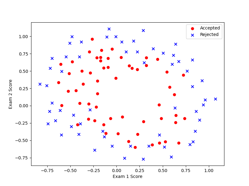
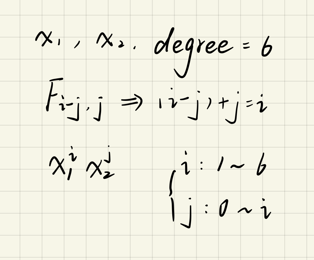
2.2 Feature mapping
目的:为每组数据创造更多的特征,这样h(theta)就可以是高阶的函数,才可能将上述的这种数据集进行分类。

main.py
import pandas as pd
import numpy as np
from plot import *  # 绘图

data = pd.read_csv('ex2data2.txt', header=None, names=['Exam1', 'Exam2', 'Accepted'])
data.insert(3, 'Ones', 1)
degree = 6  # 设置最高到6次幂
for i in range(1, degree + 1):
    for j in range(0, i + 1):
        data['F' + str(i - j) + str(j)] = np.power(data['Exam1'], i - j) * np.power(data['Exam2'], j)
# drop函数指删除行(axis=0 默认)或列(axis=1),inplace=True(默认为False)则原数组被替换
data.drop('Exam1', axis=1, inplace=True)
data.drop('Exam2', axis=1, inplace=True)
print(data.head())
#    Accepted  Ones       F10      F01  ...       F33       F24       F15       F06
# 0         1     1  0.051267  0.69956  ...  0.000046  0.000629  0.008589  0.117206
# 1         1     1 -0.092742  0.68494  ... -0.000256  0.001893 -0.013981  0.103256
# 2         1     1 -0.213710  0.69225  ... -0.003238  0.010488 -0.033973  0.110047
# 3         1     1 -0.375000  0.50219  ... -0.006679  0.008944 -0.011978  0.016040
# 4         1     1 -0.513250  0.46564  ... -0.013650  0.012384 -0.011235  0.010193
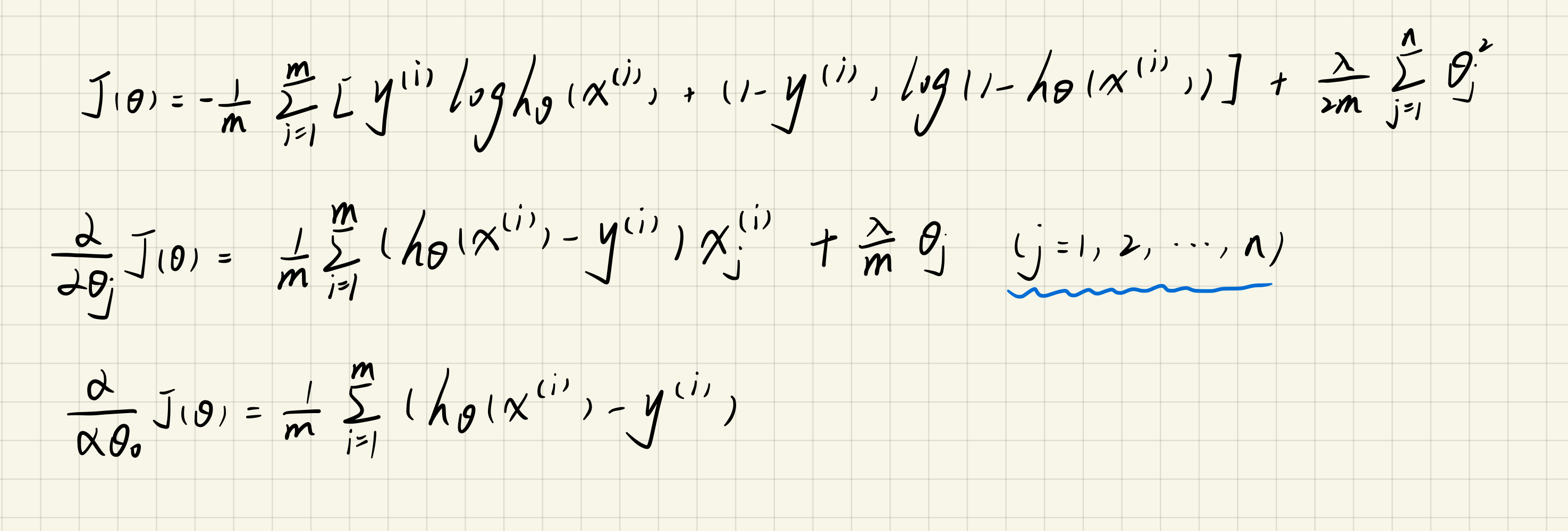
2.3 Cost function and gradient
注意:theta0不需要正则化
sigmoid.py
import numpy as np

def Sigmoid(z):
    return 1 / (1 + np.exp(-z))
costReg.py
import numpy as np
from sigmoid import *  # sigmoid函数

def costReg(theta, X, y, alpha):
    theta = np.matrix(theta)
    X = np.matrix(X)
    y = np.matrix(y)
    c1 = np.multiply(y, np.log(Sigmoid(X * theta.T)))
    c2 = np.multiply(1 - y, np.log(1 - Sigmoid(X * theta.T)))
    reg = (alpha / (2 * len(X))) * np.sum(np.power(theta[1:, :], 2))
    return -np.sum(c1 + c2) / len(X) + reg
main.py
import pandas as pd
import numpy as np
from plot import *  # 绘图
from costReg import *  # 代价函数

data = pd.read_csv('ex2data2.txt', header=None, names=['Exam1', 'Exam2', 'Accepted'])
data.insert(3, 'Ones', 1)
degree = 6  # 设置最高到6次幂
for i in range(1, degree + 1):
    for j in range(0, i + 1):
        data['F' + str(i - j) + str(j)] = np.power(data['Exam1'], i - j) * np.power(data['Exam2'], j)
# drop函数指删除行(axis=0 默认)或列(axis=1),inplace=True(默认为False)则原数组被替换
data.drop('Exam1', axis=1, inplace=True)
data.drop('Exam2', axis=1, inplace=True)

# 初始化
cols = data.shape[1]
X = data.iloc[:, 1:cols].values
y = data.iloc[:, 0:1].values
theta = np.zeros(X.shape[1])
learningRate = 1
print(costReg(theta, X, y, learningRate))  # 0.6931471805599454
gradientReg.py
import numpy as np
from sigmoid import *

def gradientReg(theta, X, y, alpha):
    theta = np.matrix(theta)
    X = np.matrix(X)
    y = np.matrix(y)
    m = len(X)
    para_theta_num = theta.shape[1]
    grad = np.zeros(para_theta_num)
    for i in range(para_theta_num):
        if i == 0:
            grad[i] = np.sum(Sigmoid(X * theta.T) - y) / m
        else:
            grad[i] = ((Sigmoid(X * theta.T) - y).T * X[:, i] + alpha * theta[0, i]) / m
    return grad
2.4 Learning parameters using fminunc
main.py
import pandas as pd
import numpy as np
import scipy.optimize as opt  # scipy优化算法
from plot import *  # 绘图
from costReg import *  # 代价函数
from gradientReg import *  # 梯度下降

data = pd.read_csv('ex2data2.txt', header=None, names=['Exam1', 'Exam2', 'Accepted'])
data.insert(3, 'Ones', 1)
degree = 6  # 设置最高到6次幂
for i in range(1, degree + 1):
    for j in range(0, i + 1):
        data['F' + str(i - j) + str(j)] = np.power(data['Exam1'], i - j) * np.power(data['Exam2'], j)
# drop函数指删除行(axis=0 默认)或列(axis=1),inplace=True(默认为False)则原数组被替换
data.drop('Exam1', axis=1, inplace=True)
data.drop('Exam2', axis=1, inplace=True)

# 初始化
cols = data.shape[1]
X = data.iloc[:, 1:cols].values
y = data.iloc[:, 0:1].values
theta = np.zeros(X.shape[1])
learningRate = 1
result = opt.fmin_tnc(func=costReg, x0=theta, args=(X, y, learningRate), fprime=gradientReg)
print(result[0])
# [ 1.27422017  0.62478647  1.18590374 -2.02173832 -0.91708237 -1.41319142
#   0.12444368 -0.36770513 -0.36458178 -0.18067781 -1.46506518 -0.06288695
#  -0.61999793 -0.27174432 -1.20129286 -0.23663767 -0.20901438 -0.05490414
#  -0.27804406 -0.2927691  -0.46790792 -1.04396474  0.02082845 -0.29638538
#   0.00961557 -0.32917183 -0.13804211 -0.93550829]
2.5 Evaluate
predict.py
from sigmoid import *

def Predict(theta, X):
    probability = Sigmoid(X * theta.T)
    return [1 if x >= 0.5 else 0 for x in probability]
main.py
import pandas as pd
import numpy as np
import scipy.optimize as opt  # scipy优化算法
from plot import *  # 绘图
from costReg import *  # 代价函数
from gradientReg import *  # 梯度下降
from predict import *

data = pd.read_csv('ex2data2.txt', header=None, names=['Exam1', 'Exam2', 'Accepted'])
data.insert(3, 'Ones', 1)
degree = 6  # 设置最高到6次幂
for i in range(1, degree + 1):
    for j in range(0, i + 1):
        data['F' + str(i - j) + str(j)] = np.power(data['Exam1'], i - j) * np.power(data['Exam2'], j)
# drop函数指删除行(axis=0 默认)或列(axis=1),inplace=True(默认为False)则原数组被替换
data.drop('Exam1', axis=1, inplace=True)
data.drop('Exam2', axis=1, inplace=True)

# 初始化
cols = data.shape[1]
X = data.iloc[:, 1:cols].values
y = data.iloc[:, 0:1].values
theta = np.zeros(X.shape[1])
learningRate = 1
result = opt.fmin_tnc(func=costReg, x0=theta, args=(X, y, learningRate), fprime=gradientReg)
theta = np.matrix(result[0])
predictions = Predict(theta, X)
correct = [1 if (a == 1 and b == 1) or (a == 0 and b == 0) else 0 for (a, b) in zip(predictions, y)]
accuracy = sum(correct) % len(correct)
print('accuracy={0}%'.format(accuracy))  # accuracy=98%
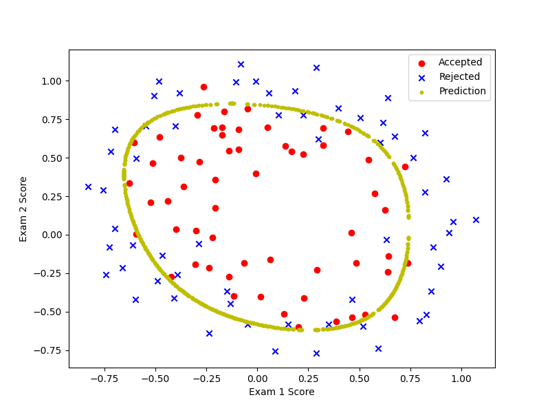
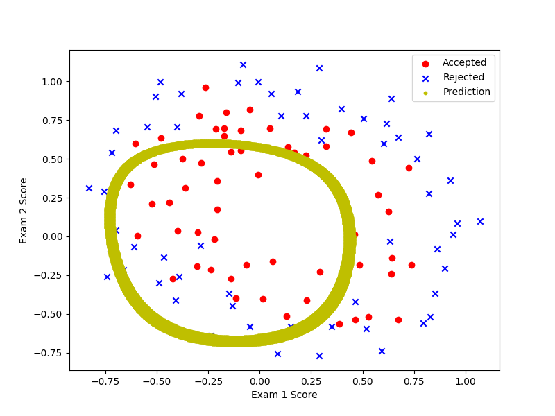
2.6 Plotting the decision boundary
注意:在find_decision_boundary中找到theta转置乘X接近于0的情况,这时候的x1与x2特征值一个视为x一个视为y,再画出决策边界。
decisionBoundary.py
import numpy as np
import pandas as pd

def h_theta(theta, x1, x2):
    degree = 6
    res = theta[0, 0]
    place = 0
    for i in range(1, degree + 1):
        for j in range(0, i + 1):
            res += np.power(x1, i - j) * np.power(x2, j) * theta[0, place + 1]
            place += 1
    return res

def find_decision_boundary(theta):
    t1 = np.linspace(-1, 1.5, 1000)
    t2 = np.linspace(-1, 1.5, 1000)
    coordinates = [(x, y) for x in t1 for y in t2]
    x_cord, y_cord = zip(*coordinates)  # zip(*..)表示解压
    h_val = pd.DataFrame({'x1': x_cord, 'x2': y_cord})
    h_val['value'] = h_theta(theta, h_val['x1'], h_val['x2'])  # 特征x1、x2在theta下的函数值
    decision = h_val[np.abs(h_val['value']) < 2 * 10 ** -3]
    return decision.x1, decision.x2  # 返回的是函数值小于2*10的-3次方的x1与x2特征值
main.py
import pandas as pd
import numpy as np
import scipy.optimize as opt  # scipy优化算法
import matplotlib.pyplot as plt  # 可视化工具
from costReg import *  # 代价函数
from gradientReg import *  # 梯度下降
from predict import *
from decisionBoundary import *  # 决策边界

data = pd.read_csv('ex2data2.txt', header=None, names=['Exam1', 'Exam2', 'Accepted'])
data.insert(3, 'Ones', 1)
positive = data[data.Accepted.isin([1])]
negative = data[data.Accepted.isin([0])]
# 画出训练集
fig, ax = plt.subplots(figsize=(8, 6))
ax.scatter(positive['Exam1'], positive['Exam2'], c='r', marker='o', label='Accepted')
ax.scatter(negative['Exam1'], negative['Exam2'], c='b', marker='x', label='Rejected')
ax.set_xlabel('Exam 1 Score')
ax.set_ylabel('Exam 2 Score')

degree = 6  # 设置最高到6次幂
for i in range(1, degree + 1):
    for j in range(0, i + 1):
        data['F' + str(i - j) + str(j)] = np.power(data['Exam1'], i - j) * np.power(data['Exam2'], j)
# drop函数指删除行(axis=0 默认)或列(axis=1),inplace=True(默认为False)则原数组被替换
data.drop('Exam1', axis=1, inplace=True)
data.drop('Exam2', axis=1, inplace=True)

# 初始化
cols = data.shape[1]
X = data.iloc[:, 1:cols].values
y = data.iloc[:, 0:1].values
theta = np.zeros(X.shape[1])
learningRate = 1
result = opt.fmin_tnc(func=costReg, x0=theta, args=(X, y, learningRate), fprime=gradientReg)
theta = np.matrix(result[0])
predictions = Predict(theta, X)
correct = [1 if (a == 1 and b == 1) or (a == 0 and b == 0) else 0 for (a, b) in zip(predictions, y)]
accuracy = sum(correct) % len(correct)
# print('accuracy={0}%'.format(accuracy))  # accuracy=98%

# 画出决策边界
x, y = find_decision_boundary(theta)
ax.scatter(x, y, c='y', s=10, label='Prediction')
ax.legend()
plt.show()
2.7 change λ(之前用learningRate表示的)
λ=0时,即在main.py里修改为learningRate = 0,变现为过拟合(overfitting)。
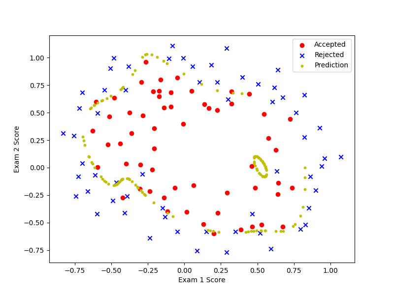
λ=100时,即在main.py里修改为learningRate = 100,变现为欠拟合(underfitting)。


 909
909


 被折叠的 条评论
为什么被折叠?
被折叠的 条评论
为什么被折叠?
 到【灌水乐园】发言


