[深度学习]pytorch实现sigmoid、softmax、交叉熵loss函数

一、实现softmax函数

$$\mathrm{Softmax}\left(z_i\right)=\frac{e^{z_i}}{{\sum }_{c=1}^C{e}^{z_c}}$$
其中$z_i$为第$i$个节点的输出值，$C$为输出节点的个数，即分类的类别个数。通过Softmax函数就可以将多分类的输出值转换为范围在[0, 1]，和为1的概率分布。

def softmax(x):
    X_exp = np.exp(x)
    partition = X_exp.sum(1, keepdims=True)
    return X_exp / partition  # 这里应用了广播机制

test_data =torch.tensor(np.random.normal(size=[10, 5]))
(softmax(test_data)-torch.nn.functional.softmax(torch.tensor(test_data), dim=-1).numpy())**2 <0.001

输出

tensor([[True, True, True, True, True],
        [True, True, True, True, True],
        [True, True, True, True, True],
        [True, True, True, True, True],
        [True, True, True, True, True],
        [True, True, True, True, True],
        [True, True, True, True, True],
        [True, True, True, True, True],
        [True, True, True, True, True],
        [True, True, True, True, True]])

二、实现sigmoid函数

Sigmoid函数由下列公式定义
$$S(x)=\frac{1}{1+e^{-x}}$$
其对x的导数可以用自身表示：$$S^{\prime }(x)=\frac{e^{-x}}{{\left(1+e^{-x}\right)}^2}=S(x)(1-S(x))$$

def sigmoid(x):
    prob_x = 1 / (1 + torch.exp(-x))
    return prob_x

test_data = torch.tensor(np.random.normal(size=[10, 5]))
(sigmoid(test_data)-torch.nn.functional.sigmoid(torch.tensor(test_data)).numpy())**2 < 0.0001

输出

tensor([[True, True, True, True, True],
        [True, True, True, True, True],
        [True, True, True, True, True],
        [True, True, True, True, True],
        [True, True, True, True, True],
        [True, True, True, True, True],
        [True, True, True, True, True],
        [True, True, True, True, True],
        [True, True, True, True, True],
        [True, True, True, True, True]])

三、实现交叉熵loss函数

CrossEntropy交叉熵损失函数
1、交叉熵损失函数经常用于分类问题中，特别是在神经网络做分类问题时，也经常使用交叉熵作为损失函数，此外，由于交叉熵涉及到计算每个类别的概率，所以交叉熵几乎每次都和sigmoid(或softmax)函数一起出现。
我们用神经网络最后一层输出的情况，来看一眼整个模型预测、获得损失和学习的流程：

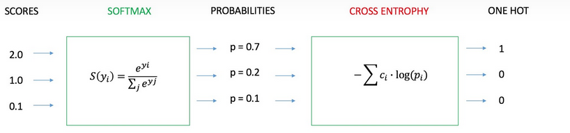
1、神经网络最后一层得到每个类别的得分scores（也叫logits）
2、该得分经过sigmoid(或softmax)函数获得概率输出；
3、模型预测的类别概率输出与真实类别的one hot形式进行交叉熵损失函数的计算。

2、Cross Entropy Loss Function（交叉熵损失函数）表达式

（1）二分类
在二分的情况下，模型最后需要预测的结果只有两种情况，对于每个类别我们的预测得到的概率为 $p$ 和 $1-p$ ，此时表达式为 $(\log$ 的底数是 $e)$ :
$$L=\frac{1}{N}\sum _i{L}_i=\frac{1}{N}\sum _i-\left[y_i\cdot \log \left(p_i\right)+\left(1-y_i\right)\cdot \log \left(1-p_i\right)\right]$$
其中:

• $y_i$ 一表示样本 $i$ 的label，正类为 1 ，负类为 0
• $p_i$ — 表示样本 $i$ 预测为正类的概率

（2）多分类
多分类的情况实际上就是对二分类的扩展:
$$L=\frac{1}{N}\sum _i{L}_i=-\frac{1}{N}\sum _i\sum _{c=1}^M{y}_{ic}\log \left(p_{ic}\right)$$其中:

• $M$ 一类别的数量
• $y_{ic}$ —符号函数（ 0或1），如果样本 $i$ 的真实类别等于$c$取1，否则取0
• $p_{ic}$ —观测样本 $i$ 属于类别 $c$ 的预测概率

（一） 实现 sigmoid 交叉熵loss函数（二分类）

def sigmoid_ce(x, label):
    loss = -np.mean(np.nan_to_num(label*np.log(x)+(1-label)*np.log(1-x)))
    return loss

test_data = np.random.normal(size=[10])
prob = torch.nn.functional.sigmoid(torch.tensor(test_data))
label = np.random.randint(0, 2, 10).astype(test_data.dtype)

torch_output = torch.mean(torch.nn.BCEWithLogitsLoss(reduction='none')(torch.tensor(test_data), torch.tensor(label)))
((torch_output-sigmoid_ce(prob,torch.tensor(label)))**2<0.00001).numpy()

（二）实现 softmax交叉熵loss函数（多分类）

（1）第一种写法

def softmax_ce(x, label):
    loss = -np.sum(np.nan_to_num(label*np.log(x)),axis=1)
    return loss

test_data = np.random.normal(size=[10, 5])
prob = torch.nn.functional.softmax(torch.tensor(test_data))

label = np.zeros_like(test_data)
label[np.arange(10), np.random.randint(0, 5, size=10)]=1.
torch_output = torch.nn.CrossEntropyLoss(reduction='none')(torch.tensor(test_data),torch.tensor(label))
((torch.mean(torch_output-softmax_ce(prob.numpy(), label))**2 < 0.0001))

输出

tensor(True)

（2）第二种写法
1）实例
创建一个数据样本y_hat，其中包含2个样本在3个类别的预测概率，以及它们对应的标签y。
有了y，我们知道在第一个样本中，第一类是正确的预测；
而在第二个样本中，第三类是正确的预测。
然后(使用y作为y_hat中概率的索引)，
我们选择第一个样本中第一个类的概率和第二个样本中第三个类的概率。

y = torch.tensor([0, 2])
y_hat = torch.tensor([[0.1, 0.3, 0.6], [0.3, 0.2, 0.5]])
y_hat[[0, 1], y]

输出

tensor([0.1000, 0.5000])

只需一行代码就可以实现交叉熵损失函数

def cross_entropy(y_hat, y):
    return - torch.log(y_hat[range(len(y_hat)), y])

cross_entropy(y_hat, y)

输出

tensor([2.3026, 0.6931])

2）实践

def softmax_ce(x, label):
    loss= - torch.log(x[range(len(x)),torch.argmax(torch.tensor(label), dim=1)])
    return loss

test_data = np.random.normal(size=[10, 5])
prob = torch.nn.functional.softmax(torch.tensor(test_data))

label = np.zeros_like(test_data)
label[np.arange(10), np.random.randint(0, 5, size=10)]=1

torch_output = torch.nn.CrossEntropyLoss(reduction='none')(torch.tensor(test_data),torch.tensor(label))
((torch.mean(torch_output-softmax_ce(prob,label))**2 < 0.0001))

输出

tensor(True)