A Fast Approximation of the Bilateral Filter using a Signal Processing Approach

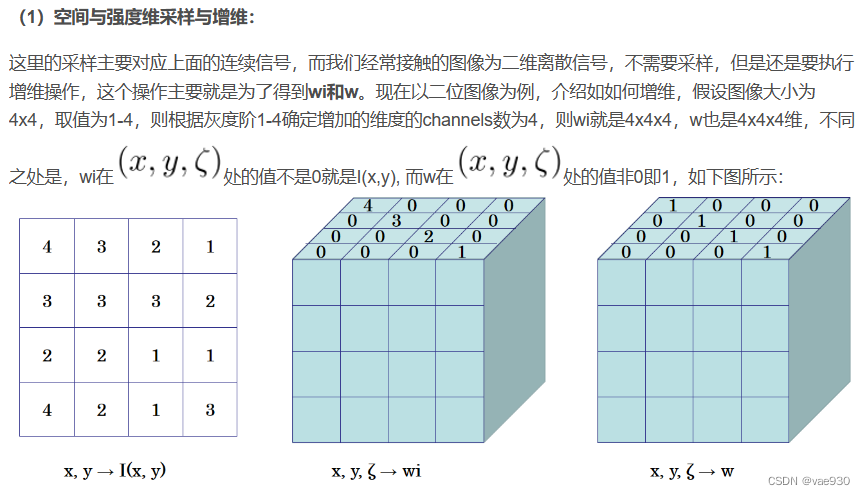
import numpy as np
import math
import scipy.signal, scipy.interpolate
import matplotlib.pyplot as plt
import cv2

def bilateral_approximation(image, sigmaS, sigmaR, samplingS=None, samplingR=None):
    # It is derived from Jiawen Chen's matlab implementation
    # The original papers and matlab code are available at http://people.csail.mit.edu/sparis/bf/

    # --------------- 原始分辨率 --------------- #
    inputHeight = image.shape[0]
    inputWidth = image.shape[1]
    sigmaS = sigmaS
    sigmaR = sigmaR
    samplingS = sigmaS if (samplingS is None) else samplingS
    samplingR = sigmaR if (samplingR is None) else samplingR
    edgeMax = np.amax(image)
    edgeMin = np.amin(image)
    edgeDelta = edgeMax - edgeMin

    # --------------- 下采样 --------------- #
    derivedSigmaS = sigmaS / samplingS
    derivedSigmaR = sigmaR / samplingR

    paddingXY = math.floor(2 * derivedSigmaS) + 1
    paddingZ = math.floor(2 * derivedSigmaR) + 1

    downsampledWidth = int(round((inputWidth - 1) / samplingS) + 1 + 2 * paddingXY)
    downsampledHeight = int(round((inputHeight - 1) / samplingS) + 1 + 2 * paddingXY)
    downsampledDepth = int(round(edgeDelta / samplingR) + 1 + 2 * paddingZ)

    wi = np.zeros((downsampledHeight, downsampledWidth, downsampledDepth))
    w = np.zeros((downsampledHeight, downsampledWidth, downsampledDepth))

    # 下采样索引
    (ygrid, xgrid) = np.meshgrid(range(inputWidth), range(inputHeight))

    dimx = np.around(xgrid / samplingS) + paddingXY
    dimy = np.around(ygrid / samplingS) + paddingXY
    dimz = np.around((image - edgeMin) / samplingR) + paddingZ

    flat_image = image.flatten()
    flatx = dimx.flatten()
    flaty = dimy.flatten()
    flatz = dimz.flatten()

    # 盒式滤波器（平均下采样）
    for k in range(dimz.size):
        image_k = flat_image[k]
        dimx_k = int(flatx[k])
        dimy_k = int(flaty[k])
        dimz_k = int(flatz[k])

        wi[dimx_k, dimy_k, dimz_k] += image_k
        w[dimx_k, dimy_k, dimz_k] += 1

    # ---------------  三维卷积 --------------- #
    # 生成卷积核
    kernelWidth = 2 * derivedSigmaS + 1
    kernelHeight = kernelWidth
    kernelDepth = 2 * derivedSigmaR + 1

    halfKernelWidth = math.floor(kernelWidth / 2)
    halfKernelHeight = math.floor(kernelHeight / 2)
    halfKernelDepth = math.floor(kernelDepth / 2)

    (gridX, gridY, gridZ) = np.meshgrid(range(int(kernelWidth)), range(int(kernelHeight)), range(int(kernelDepth)))
    # 平移，使得中心为0
    gridX -= halfKernelWidth
    gridY -= halfKernelHeight
    gridZ -= halfKernelDepth
    gridRSquared = ((gridX * gridX + gridY * gridY) / (derivedSigmaS * derivedSigmaS)) + \
                   ((gridZ * gridZ) / (derivedSigmaR * derivedSigmaR))
    kernel = np.exp(-0.5 * gridRSquared)

    # 卷积
    blurredGridData = scipy.signal.fftconvolve(wi, kernel, mode='same')
    blurredGridWeights = scipy.signal.fftconvolve(w, kernel, mode='same')

    # ---------------  divide --------------- #
    blurredGridWeights = np.where(blurredGridWeights == 0, -2, blurredGridWeights)  # avoid divide by 0, won't read there anyway
    normalizedBlurredGrid = blurredGridData / blurredGridWeights
    normalizedBlurredGrid = np.where(blurredGridWeights < -1, 0, normalizedBlurredGrid)  # put 0s where it's undefined

    # --------------- 上采样 --------------- #
    (ygrid, xgrid) = np.meshgrid(range(inputWidth), range(inputHeight))

    # 上采样索引
    dimx = (xgrid / samplingS) + paddingXY
    dimy = (ygrid / samplingS) + paddingXY
    dimz = (image - edgeMin) / samplingR + paddingZ

    out_image = scipy.interpolate.interpn((range(normalizedBlurredGrid.shape[0]),
                                           range(normalizedBlurredGrid.shape[1]),
                                           range(normalizedBlurredGrid.shape[2])),
                                          normalizedBlurredGrid,
                                          (dimx, dimy, dimz))
    return out_image

if __name__ == "__main__":
    image = cv2.imread('lena512.bmp', 0)
    mean_image = bilateral_approximation(image, sigmaS=64, sigmaR=32, samplingS=32, samplingR=16)
    plt.figure()
    plt.subplot(121)
    plt.axis('off')
    plt.imshow(image, cmap='gray')
    plt.subplot(122)
    plt.axis('off')
    plt.imshow(mean_image, cmap='gray')
    plt.show()
 

关于python的代码。

1. 简介
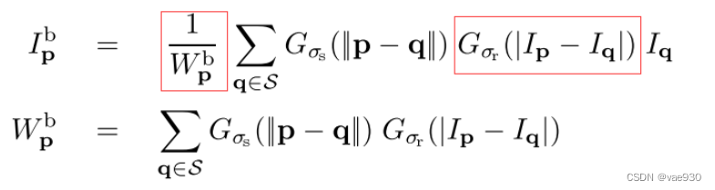
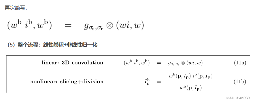
双边滤波非常有用，但速度很慢，因为它是非线性的，传统的加速算法例如在FFT之后执行卷积，是不适用的。本文提出了对双边滤波的新解释，即高维卷积，然后是两个非线性操作。其基本思想就是将非线性的双边滤波改成可分离的线性操作和非线性操作。换句话说，原来的双边滤波在图像不同位置应用不同的权重，也就是位移改变卷积，他们通过增加一个维度，也就是将灰度值作为一个新的维度，将双边滤波表达成3D空间中的线性位移不变卷积，最后再执行非线性的归一化操作。

 

2. 原理

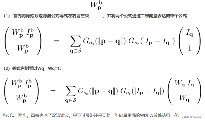
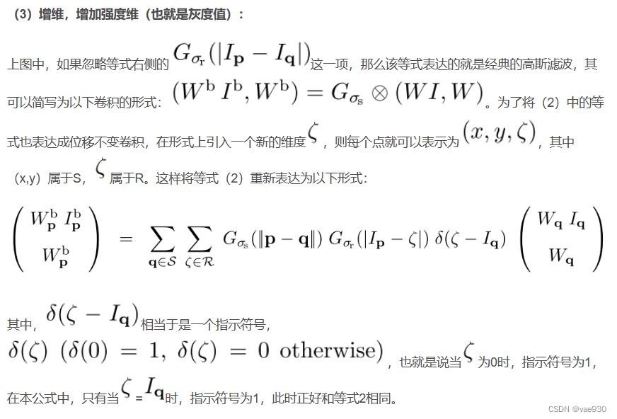
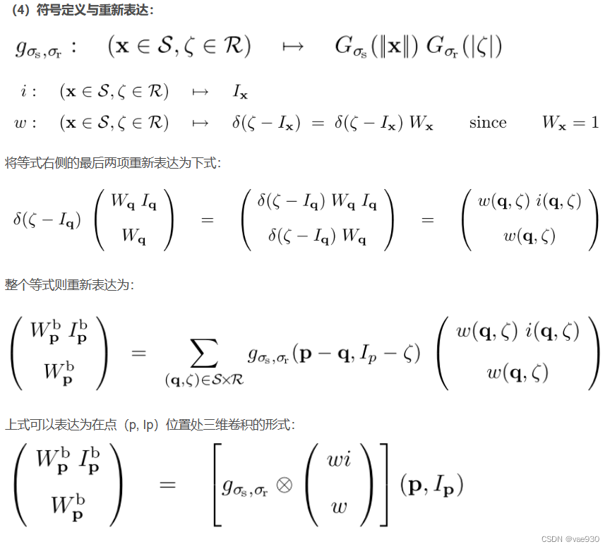
2.1 公式推导

 

 

 

 

2.2 图文并茂模式

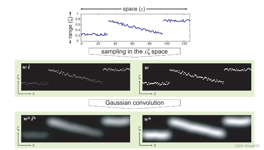
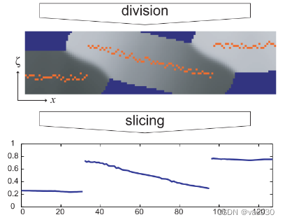
先上一张大图感受一下整个过程，以一维信号为例：

 

 

 

 

 

 

————————————————
版权声明：本文为CSDN博主「Nick Blog」的原创文章，遵循CC 4.0 BY-SA版权协议，转载请附上原文出处链接及本声明。
原文链接：https://blog.csdn.net/xijuezhu8128/article/details/111304006