scikit-learn笔记

1.过拟台和灾拟合

过拟合 是指模型能很好地拟合训练样本，但对新数据的预测准确性很 差。

欠拟合是指模型不能很好地拟合训练样本，且对新数据的预测准确性也不好。

欠拟合（ underfitting ），也称为高偏差（ high bias ）

过拟合（ overfitting ），也称为高方差（ high variance)

%matplotlib inline
import matplotlib.pyplot as plt
import numpy as np

# 设置所需要的点数
n_dots = 20

# x轴的坐标
# [0, 1] 之间创建 20 个点
x = np.linspace(0, 1, n_dots)
# y轴坐标：训练样本
y = np.sqrt(x) + 0.2*np.random.rand(n_dots) - 0.1;
def plot_polynomial_fit(x, y, order):
    p = np.poly1d(np.polyfit(x, y, order))

    # 画出拟合出来的多项式所表达的曲线以及原始的点
    t = np.linspace(0, 1, 200)
    # 设置虚线和实线分别表示的模型
    plt.plot(x, y, 'ro', t, p(t), '-', t, np.sqrt(t), 'r--')
    return p
# figsize:指定figure的宽和高，单位为英寸；
plt.figure(figsize=(18, 4))
titles = ['Under Fitting', 'Fitting', 'Over Fitting']
models = [None, None, None]
for index, order in enumerate([1, 3, 10]):
    # 创建多个子图（此处为三个）
    plt.subplot(1, 3, index + 1)
    models[index] = plot_polynomial_fit(x, y, order)
    # 设置图像的标题
    plt.title(titles[index], fontsize=20)

2.成本函数

成本是衡 量模型与 训练样本符合程度的指标。

成本 是针对 所有的训 练样 本，模型拟合出来的值与训练样本的真实值的 误差平均值 而成 本函数就是 成本与 模型参 数的函 数关系。

一个数据集可能有多 个模型可以用来拟合它，而 个模型有无穷多个模型参数，针对特定的数据集和特定的模型，只有一个模型参数能最好地拟合这个数据集，这就是模型 模型参数的关系。

总结起来，针对一 个数据 ，我们可以选择很多 个模型来拟合 数据，一 旦选定了某个模型，就需要从这个模型的无 穷多 个参数里 找出一 个最优的参数，使得成本函数的值最小。

3.模型准确性

测试数据集 的成本，即 Jt est()   是评估模型准确性的最直观的指标， Jtest(  ）值越小说明模型预测出来的值与实际值差异越小，对新数据的预测准确性就越好。

针对上文我文 介绍的线性回归算法，可以使用下面的公式计算测试数据集的误差，其中m是测试数据集的的个数：

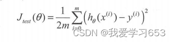
1) 模型性能的不同表述方式

 在scikit-leam 里，不使用成本函数来表达模型的性能，而使用分数来表达，这个分数总是在【0，1】间， 数值越大说明模型的准确性越好。

模型分数（准确性〉与成本成反比 即分数越大，准确性越高，误差越小，成本越低 反之，分数越小，准确性越低，误 越大，成本越高。

2交叉验证数据集

把数据集分成 份， 分别是训练数据集 交叉验证数据集测试数据集，推荐比例是6 : 2 : 2。

我们把数据集分成训练数据集和测试数据集。在模型选择时，我们使用训练数据集来训练算法参数，用 交叉验证数据集来验证参数。选择交叉验证数据集的成本 J 最小的多项式来作为数据拟合模型，最后再用测试数据集来测试选择出来的模型针对测试数据集的准确性。  

4.学习曲线

如果数据集的大小为 m ，则通过下面的流程即可画出 学习曲线:

·把数 据集分成训练数据集矛 l:J 交叉验证数据集。

·取训练 数据集的 0% 作为训 练样本，训练出模型参数。

·使用 交叉验证数据集来计算训练出来的模型的准确性。

·以训练 数据集的准确性，交叉验证的准确性作为纵坐标，训练数据集个数作为横坐

标，在坐标轴上画出上述步骤计算出来的模型准确性

·训练 数据集增加 10% ，跳到步骤 继续执行，直到训练数据集大小为 100% 为止。

学习曲线要表达的内容是，当训练数据集增加时，模型对训练数据集拟合的准确性以

及对交叉验证数据集预测的准确性的变化规律。

1） 实例：画出学习曲线

%matplotlib inline
import matplotlib.pyplot as plt
import numpy as np
n_dots = 200

X = np.linspace(0, 1, n_dots)                   
y = np.sqrt(X) + 0.2*np.random.rand(n_dots) - 0.1;

X = X.reshape(-1, 1)
y = y.reshape(-1, 1)

   构造一 个多项式模型。

from sklearn.pipeline import Pipeline#流水线
from sklearn.preprocessing import PolynomialFeatures
from sklearn.linear_model import LinearRegression

def polynomial_model(degree=1):#阶数
    polynomial_features = PolynomialFeatures(degree=degree,
                                             include_bias=False)
    linear_regression = LinearRegression()
#     先增加多项式阶数，然后再用线性回归算法来拟合数据
    pipeline = Pipeline([("polynomial_features", polynomial_features),
                         ("linear_regression", linear_regression)])
    return pipeline
from sklearn.model_selection import learning_curve
from sklearn.model_selection import ShuffleSplit

def plot_learning_curve(estimator, title, X, y, ylim=None, cv=None,
                        n_jobs=1, train_sizes=np.linspace(.1, 1.0, 5)):
    plt.title(title)
    if ylim is not None:
        plt.ylim(*ylim)
    plt.xlabel("Training examples")
    plt.ylabel("Score")
    train_sizes, train_scores, test_scores = learning_curve(
        estimator, X, y, cv=cv, n_jobs=n_jobs, train_sizes=train_sizes)
    train_scores_mean = np.mean(train_scores, axis=1)
    train_scores_std = np.std(train_scores, axis=1)
    test_scores_mean = np.mean(test_scores, axis=1)
    test_scores_std = np.std(test_scores, axis=1)
    plt.grid()

    plt.fill_between(train_sizes, train_scores_mean - train_scores_std,
                     train_scores_mean + train_scores_std, alpha=0.1,
                     color="r")
    plt.fill_between(train_sizes, test_scores_mean - test_scores_std,
                     test_scores_mean + test_scores_std, alpha=0.1, color="g")
    plt.plot(train_sizes, train_scores_mean, 'o--', color="r",
             label="Training score")
    plt.plot(train_sizes, test_scores_mean, 'o-', color="g",
             label="Cross-validation score")

    plt.legend(loc="best")
    return plt

# 为了让学习曲线更平滑，交叉验证数据集的得分计算 10 次，每次都重新选中 20% 的数据计算一遍
cv = ShuffleSplit(n_splits=10, test_size=0.2, random_state=0)
titles = ['Learning Curves (Under Fitting)',
          'Learning Curves',
          'Learning Curves (Over Fitting)']
degrees = [1, 3, 10]

plt.figure(figsize=(18, 4))
for i in range(len(degrees)):
    plt.subplot(1, 3, i + 1)
    plot_learning_curve(polynomial_model(degrees[i]), titles[i], X, y, ylim=(0.75, 1.01), cv=cv)

plt.show()

当发 生高偏差时，增加训 练样本数 不会对算法准确性有较大的改善。

2）过拟合和欠拟合的特征

总结过拟 和欠拟合的特点如下

过拟合：模型对训练 数据集的 准确性比较 其成本 J 比较低, 对交叉验证数据集的准确性比较低 成本J   比较高。

欠拟合： 模型对训练数据集的准确性 较低，其成本 J   较高, 对交叉验证数据集的准确性也比较低，其成本 Jcv 比较高。

一个好的机 器学习算法应该是对训练数据集准确性高、成本低，即较准确 地拟 合数据同时对交叉验证数据集准确性高 、成本低、误差小  ，即对未知数据有良好的预测性。

5.算法模型性能优化

如果是过拟合，可以采取的措施如下：

1）获取更多的训练、数据：

2）减少输入的特征数量：

3） 增加有价值的特征：

4）增加多项式特征：

6.查准率和召回率

有时候，模型准确性并不能评价一个算法的好坏。我们引入了另外两个概念，查准率 (Precision ）和召 率（Recall 。还是 以癌症筛查为例：

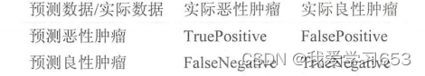
查准率和］召回率的定义如下：

 

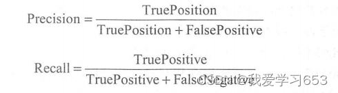
在scikit-leam 里，评估模型性能的算法都在 klean. metrics 里。其中，计算查准率 和召回率的 API 分别为 sklean.metrics precision_ score （）和 sk l ean .metr ics.recall _ score （）

 

7.F1 Score

我们引入了 F1Sco re 概念：

 

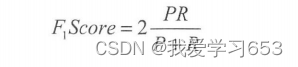
其中 是查准率， 是召回率。这样就可以用 个数值直接判断哪个算法性能更好。

典型地，如果查准率或召回率有 个为 ，那么 F1Score 将会为 。而理想的情况下，查准

率和召回率都为1，  算出来的 F Score 为1。

在sc ikit-learn 里，计算F Score  的函数是 skl ean. m etrics. fl_ score （）。