Sample space

omipus

已于 2022-12-17 21:07:24 修改

阅读量152

点赞数

分类专栏： Reference 文章标签：算法

于 2022-10-08 21:33:19 首次发布

本文链接：https://blog.csdn.net/qq_66485519/article/details/127215492

版权

Reference 专栏收录该内容

581 篇文章 5 订阅

订阅专栏

In probability theory, the sample space (also called sample description space or possibility space) of an experiment or random trial is the set of all possible outcomes or results of that experiment. A sample space is usually denoted using set notation, and the possible ordered outcomes, or sample points, are listed as elements in the set. It is common to refer to a sample space by the labels $S$ , $Ω$ , or $U$ (for “universal set”). The elements of a sample space may be numbers, words, letters, or symbols. They can also be finite, countably infinite, or uncountably infinite.

A subset of the sample space is an event, denoted by $E$ . If the outcome of an experiment is included in $E$ , then event $E$ has occurred.

For example, if the experiment is tossing a single coin, the sample space is the set $\{H,T\}$ , where the outcome $H$ means that the coin is heads and the outcome $T$ means that the coin is tails. The possible events are $E=\{H\}$ , $E=\{T\}$ , and $E=\{H,T\}$ . For tossing two coins, the sample space is $\{HH,HT,TH,TT\}$ , where the outcome is $HH$ if both coins are heads, $HT$ if the first coin is heads and the second is tails, $TH$ if the first coin is tails and the second is heads, and $TT$ if both coins are tails. The event that at least one of the coins is heads is given by $E=\{HH,HT,TH\}$ .

For tossing a single six-sided die one time, where the result of interest is the number of pips facing up, the sample space is $\{1,2,3,4,5,6\}$ .

A well-defined, non-empty sample space $S$ is one of three components in a probabilistic model (a probability space). The other two basic elements are: a well-defined set of possible events (an event space), which is typically the power set of $S$ if $S$ is discrete or a σ-algebra on $S$ if it is continuous, and a probability assigned to each event (a probability measure function).

A sample space can be represented visually by a rectangle, with the outcomes of the sample space denoted by points within the rectangle. The events may be represented by ovals, where the points enclosed within the oval make up the event.

在这里插入图片描述

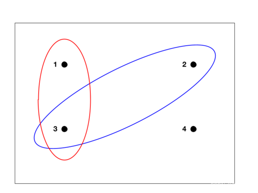
A visual representation of a finite sample space and events. The red oval is the event that a number is odd, and the blue oval is the event that a number is prime.

1 Conditions of a sample space
2 Multiple sample spaces
3 Equally likely outcomes
- 3.1 Simple random sample
4 Infinitely large sample spaces
5 See also
6 References
7 External links

1 Conditions of a sample space

A set $\Omega$ with outcomes $s_{1},s_{2},\ldots ,s_{n}$ (i.e. $\Omega =\{s_{1},s_{2},\ldots ,s_{n}\}$ ) must meet some conditions in order to be a sample space:

The outcomes must be mutually exclusive, i.e. if $s_{j}$ occurs, then no other $s_{i}$ will take place, $\forall i,j=1,2,\ldots ,n\quad i\neq j$
The outcomes must be collectively exhaustive, i.e. on every experiment (or random trial) there will always take place some outcome $s_{i}\in \Omega$ for $i\in \{1,2,\ldots ,n\}$
The sample space ( $\Omega$ ) must have the right granularity depending on what the experimenter is interested in. Irrelevant information must be removed from the sample space and the right abstraction must be chosen.

For instance, in the trial of tossing a coin, one possible sample space is $\Omega _{1}=\{H,T\}$ , where $H$ is the outcome where the coin lands heads and $T$ is for tails. Another possible sample space could be $\Omega _{2}=\{(H,R),(H,NR),(T,R),(T,NR)\}$ . Here, $R$ denotes a rainy day and $NR$ is a day where it is not raining. For most experiments, $\Omega _{1}$ would be a better choice than $\Omega _{2}$ , as an experimenter likely do not care about how the weather affects the coin toss.

2 Multiple sample spaces

For many experiments, there may be more than one plausible sample space available, depending on what result is of interest to the experimenter. For example, when drawing a card from a standard deck of fifty-two playing cards, one possibility for the sample space could be the various ranks (Ace through King), while another could be the suits (clubs, diamonds, hearts, or spades). A more complete description of outcomes, however, could specify both the denomination and the suit, and a sample space describing each individual card can be constructed as the Cartesian product of the two sample spaces noted above (this space would contain fifty-two equally likely outcomes). Still other sample spaces are possible, such as right-side up or upside down, if some cards have been flipped when shuffling.

3 Equally likely outcomes

Main article: Equally likely outcomes

Some treatments of probability assume that the various outcomes of an experiment are always defined so as to be equally likely. For any sample space with $N$ equally likely outcomes, each outcome is assigned the probability ${\frac {1}{N}}$ . However, there are experiments that are not easily described by a sample space of equally likely outcomes—for example, if one were to toss a thumb tack many times and observe whether it landed with its point upward or downward, there is no physical symmetry to suggest that the two outcomes should be equally likely.

Though most random phenomena do not have equally likely outcomes, it can be helpful to define a sample space in such a way that outcomes are at least approximately equally likely, since this condition significantly simplifies the computation of probabilities for events within the sample space. If each individual outcome occurs with the same probability, then the probability of any event becomes simply:
$\mathrm {P} ({\text{event}})={\frac {\text{number of outcomes in event}}{\text{number of outcomes in sample space}}}$

For example, if two fair six-sided dice are thrown to generate two uniformly distributed integers, $D_{1}$ and $D_{2}$ , each in the range from $1$ to $6$ , inclusive, the $36$ possible ordered pairs of outcomes $(D_{1},D_{2})$ constitute a sample space of equally likely events. In this case, the above formula applies, such as calculating the probability of a particular sum of the two rolls in an outcome. The probability of the event that the sum $D_{1}+D_{2}$ is five is ${\frac {4}{36}}$ , since four of the thirty-six equally likely pairs of outcomes sum to five.

If the sample space was the all of the possible sums obtained from rolling two six-sided dice, the above formula can still be applied because the dice rolls are fair, but the number of outcomes in a given event will vary. A sum of two can occur with the outcome $\{(1,1)\}$ , so the probability is ${\frac {1}{36}}$ . For a sum of seven, the outcomes in the event are $\{(1,6),(6,1),(2,5),(5,2),(3,4),(4,3)\}$ , so the probability is ${\frac {6}{36}}$ .

在这里插入图片描述

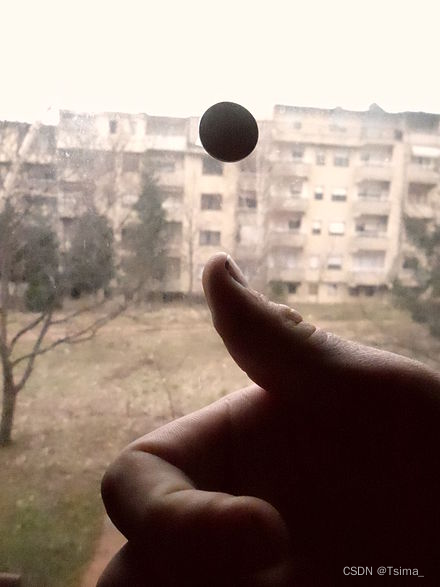
Flipping a coin leads to a sample space composed of two outcomes that are almost equally likely.

在这里插入图片描述

Up or down? Flipping a brass tack leads to a sample space composed of two outcomes that are not equally likely.

3.1 Simple random sample

Main article: Simple random sample

In statistics, inferences are made about characteristics of a population by studying a sample of that population’s individuals. In order to arrive at a sample that presents an unbiased estimate of the true characteristics of the population, statisticians often seek to study a simple random sample—that is, a sample in which every individual in the population is equally likely to be included. The result of this is that every possible combination of individuals who could be chosen for the sample has an equal chance to be the sample that is selected (that is, the space of simple random samples of a given size from a given population is composed of equally likely outcomes).

4 Infinitely large sample spaces

In an elementary approach to probability, any subset of the sample space is usually called an event. However, this gives rise to problems when the sample space is continuous, so that a more precise definition of an event is necessary. Under this definition only measurable subsets of the sample space, constituting a $σ$ -algebra over the sample space itself, are considered events.

An example of an infinitely large sample space is measuring the lifetime of a light bulb. The corresponding sample space would be $[0, \infty)$ .