Ellipse

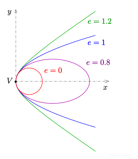
In mathematics, an ellipse is a plane curve surrounding two focal points, such that for all points on the curve, the sum of the two distances to the focal points is a constant. It generalizes a circle, which is the special type of ellipse in which the two focal points are the same. The elongation of an ellipse is measured by its eccentricity {\displaystyle e}e, a number ranging from {\displaystyle e=0}e=0 (the limiting case of a circle) to {\displaystyle e=1}e=1 (the limiting case of infinite elongation, no longer an ellipse but a parabola).

An ellipse has a simple algebraic solution for its area, but only approximations for its perimeter (also known as circumference), for which integration is required to obtain an exact solution.

Analytically, the equation of a standard ellipse centered at the origin with width {\displaystyle 2a}2a and height {\displaystyle 2b}2b is:

{\displaystyle {\frac {x^{2}}{a{2}}}+{\frac {y^{2}}{b{2}}}=1.}{\displaystyle {\frac {x^{2}}{a{2}}}+{\frac {y^{2}}{b{2}}}=1.}
Assuming {\displaystyle a\geq b}a \ge b, the foci are {\displaystyle (\pm c,0)}{\displaystyle (\pm c,0)} for {\textstyle c={\sqrt {a^{2}-b{2}}}}{\textstyle c={\sqrt {a^{2}-b{2}}}}. The standard parametric equation is:

{\displaystyle (x,y)=(a\cos(t),b\sin(t))\quad {\text{for}}\quad 0\leq t\leq 2\pi .}{\displaystyle (x,y)=(a\cos(t),b\sin(t))\quad {\text{for}}\quad 0\leq t\leq 2\pi .}
Ellipses are the closed type of conic section: a plane curve tracing the intersection of a cone with a plane (see figure). Ellipses have many similarities with the other two forms of conic sections, parabolas and hyperbolas, both of which are open and unbounded. An angled cross section of a cylinder is also an ellipse.

An ellipse may also be defined in terms of one focal point and a line outside the ellipse called the directrix: for all points on the ellipse, the ratio between the distance to the focus and the distance to the directrix is a constant. This constant ratio is the above-mentioned eccentricity:

{\displaystyle e={\frac {c}{a}}={\sqrt {1-{\frac {b^{2}}{a{2}}}}}.}{\displaystyle e={\frac {c}{a}}={\sqrt {1-{\frac {b^{2}}{a{2}}}}}.}
Ellipses are common in physics, astronomy and engineering. For example, the orbit of each planet in the Solar System is approximately an ellipse with the Sun at one focus point (more precisely, the focus is the barycenter of the Sun–planet pair). The same is true for moons orbiting planets and all other systems of two astronomical bodies. The shapes of planets and stars are often well described by ellipsoids. A circle viewed from a side angle looks like an ellipse: that is, the ellipse is the image of a circle under parallel or perspective projection. The ellipse is also the simplest Lissajous figure formed when the horizontal and vertical motions are sinusoids with the same frequency: a similar effect leads to elliptical polarization of light in optics.

The name, ἔλλειψις (élleipsis, “omission”), was given by Apollonius of Perga in his Conics.

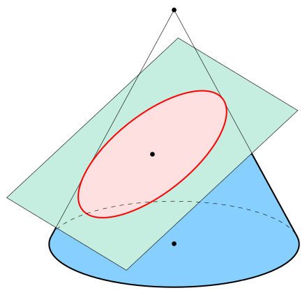
An ellipse (red) obtained as the intersection of a cone with an inclined plane.

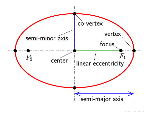
Ellipse: notations

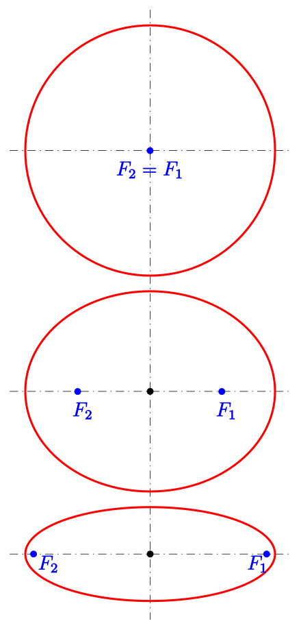
Ellipses: examples with increasing eccentricity

1 Definition as locus of points

An ellipse can be defined geometrically as a set or locus of points in the Euclidean plane:

Given two fixed points {\displaystyle F_{1},F_{2}}F_{1},F_{2} called the foci and a distance {\displaystyle 2a}2a which is greater than the distance between the foci, the ellipse is the set of points {\displaystyle P}P such that the sum of the distances {\displaystyle |PF_{1}|,\ |PF_{2}|}{\displaystyle |PF_{1}|,\ |PF_{2}|} is equal to {\displaystyle 2a}2a:{\displaystyle E=\left{P\in \mathbb {R} ^{2},\mid ,|PF_{2}|+|PF_{1}|=2a\right}\ .}{\displaystyle E=\left{P\in \mathbb {R} ^{2},\mid ,|PF_{2}|+|PF_{1}|=2a\right}\ .}
The midpoint {\displaystyle C}C of the line segment joining the foci is called the center of the ellipse. The line through the foci is called the major axis, and the line perpendicular to it through the center is the minor axis. The major axis intersects the ellipse at two vertices {\displaystyle V_{1},V_{2}}{\displaystyle V_{1},V_{2}}, which have distance {\displaystyle a}a to the center. The distance {\displaystyle c}c of the foci to the center is called the focal distance or linear eccentricity. The quotient {\displaystyle e={\tfrac {c}{a}}}{\displaystyle e={\tfrac {c}{a}}} is the eccentricity.

The case {\displaystyle F_{1}=F_{2}}{\displaystyle F_{1}=F_{2}} yields a circle and is included as a special type of ellipse.

The equation {\displaystyle |PF_{2}|+|PF_{1}|=2a}{\displaystyle |PF_{2}|+|PF_{1}|=2a} can be viewed in a different way (see figure):

If {\displaystyle c_{2}}c_{2} is the circle with center {\displaystyle F_{2}}F_{2} and radius {\displaystyle 2a}2a, then the distance of a point {\displaystyle P}P to the circle {\displaystyle c_{2}}c_{2} equals the distance to the focus {\displaystyle F_{1}}F_{1}:
{\displaystyle |PF_{1}|=|Pc_{2}|.}{\displaystyle |PF_{1}|=|Pc_{2}|.}
{\displaystyle c_{2}}c_{2} is called the circular directrix (related to focus {\displaystyle F_{2}}F_{2}) of the ellipse.[1][2] This property should not be confused with the definition of an ellipse using a directrix line below.

Using Dandelin spheres, one can prove that any section of a cone with a plane is an ellipse, assuming the plane does not contain the apex and has slope less than that of the lines on the cone.

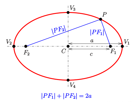
Ellipse: definition by sum of distances to foci

Ellipse: definition by focus and circular directrix

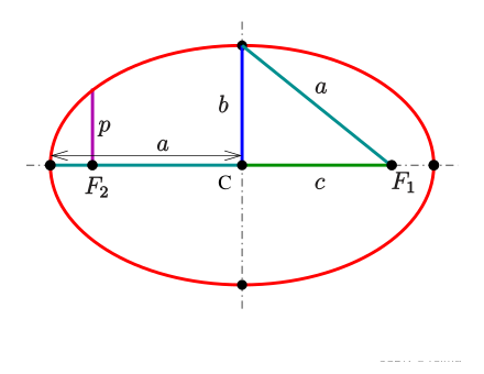
Shape parameters:
a: semi-major axis,
b: semi-minor axis,
c: linear eccentricity,
p: semi-latus rectum (usually {\displaystyle \ell }\ell ).

2 In Cartesian coordinates

2.1 Standard equation

The standard form of an ellipse in Cartesian coordinates assumes that the origin is the center of the ellipse, the x-axis is the major axis, and:

the foci are the points {\displaystyle F_{1}=(c,,0),\ F_{2}=(-c,,0)}{\displaystyle F_{1}=(c,,0),\ F_{2}=(-c,,0)},
the vertices are {\displaystyle V_{1}=(a,,0),\ V_{2}=(-a,,0)}{\displaystyle V_{1}=(a,,0),\ V_{2}=(-a,,0)}.
For an arbitrary point {\displaystyle (x,y)}(x,y) the distance to the focus {\displaystyle (c,0)}(c,0) is {\textstyle {\sqrt {(x-c)^{2}+y{2}}}}{\textstyle {\sqrt {(x-c)^{2}+y{2}}}} and to the other focus {\textstyle {\sqrt {(x+c)^{2}+y{2}}}}{\textstyle {\sqrt {(x+c)^{2}+y{2}}}}. Hence the point {\displaystyle (x,,y)}{\displaystyle (x,,y)} is on the ellipse whenever:

{\displaystyle {\sqrt {(x-c)^{2}+y{2}}}+{\sqrt {(x+c)^{2}+y{2}}}=2a\ .}{\displaystyle {\sqrt {(x-c)^{2}+y{2}}}+{\sqrt {(x+c)^{2}+y{2}}}=2a\ .}
Removing the radicals by suitable squarings and using {\displaystyle b^{2}=a{2}-c^{2}}{\displaystyle b^{2}=a{2}-c^{2}} (see diagram) produces the standard equation of the ellipse:[3]

{\displaystyle {\frac {x^{2}}{a{2}}}+{\frac {y^{2}}{b{2}}}=1,}{\displaystyle {\frac {x^{2}}{a{2}}}+{\frac {y^{2}}{b{2}}}=1,}
or, solved for y:

{\displaystyle y=\pm {\frac {b}{a}}{\sqrt {a^{2}-x{2}}}=\pm {\sqrt {\left(a^{2}-x{2}\right)\left(1-e^{2}\right)}}.}{\displaystyle y=\pm {\frac {b}{a}}{\sqrt {a^{2}-x{2}}}=\pm {\sqrt {\left(a^{2}-x{2}\right)\left(1-e^{2}\right)}}.}
The width and height parameters {\displaystyle a,;b}{\displaystyle a,;b} are called the semi-major and semi-minor axes. The top and bottom points {\displaystyle V_{3}=(0,,b),;V_{4}=(0,,-b)}{\displaystyle V_{3}=(0,,b),;V_{4}=(0,,-b)} are the co-vertices. The distances from a point {\displaystyle (x,,y)}{\displaystyle (x,,y)} on the ellipse to the left and right foci are {\displaystyle a+ex}{\displaystyle a+ex} and {\displaystyle a-ex}{\displaystyle a-ex}.

It follows from the equation that the ellipse is symmetric with respect to the coordinate axes and hence with respect to the origin.

2.2 Parameters

2.2.1 Principal axes

Throughout this article, the semi-major and semi-minor axes are denoted {\displaystyle a}a and {\displaystyle b}b, respectively, i.e. {\displaystyle a\geq b>0\ .}{\displaystyle a\geq b>0\ .}

In principle, the canonical ellipse equation {\displaystyle {\tfrac {x^{2}}{a{2}}}+{\tfrac {y^{2}}{b{2}}}=1}{\displaystyle {\tfrac {x^{2}}{a{2}}}+{\tfrac {y^{2}}{b{2}}}=1} may have {\displaystyle a<b}a<b (and hence the ellipse would be taller than it is wide). This form can be converted to the standard form by transposing the variable names {\displaystyle x}x and {\displaystyle y}y and the parameter names {\displaystyle a}a and {\displaystyle b.}{\displaystyle b.}

2.2.2 Linear eccentricity

This is the distance from the center to a focus: {\displaystyle c={\sqrt {a^{2}-b{2}}}}{\displaystyle c={\sqrt {a^{2}-b{2}}}}.

2.2.3 Eccentricity

The eccentricity can be expressed as:

{\displaystyle e={\frac {c}{a}}={\sqrt {1-\left({\frac {b}{a}}\right)^{2}}},}{\displaystyle e={\frac {c}{a}}={\sqrt {1-\left({\frac {b}{a}}\right)^{2}}},}
assuming {\displaystyle a>b.}{\displaystyle a>b.} An ellipse with equal axes ({\displaystyle a=b}a=b) has zero eccentricity, and is a circle.

2.2.4 Semi-latus rectum

The length of the chord through one focus, perpendicular to the major axis, is called the latus rectum. One half of it is the semi-latus rectum {\displaystyle \ell }\ell . A calculation shows:

{\displaystyle \ell ={\frac {b^{{2}}{a}}=a\left(1-e}{2}\right).}{\displaystyle \ell ={\frac {b^{{2}}{a}}=a\left(1-e}{2}\right).}[4]
The semi-latus rectum {\displaystyle \ell }\ell is equal to the radius of curvature at the vertices (see section curvature).

2.3 Tangent

An arbitrary line {\displaystyle g}g intersects an ellipse at 0, 1, or 2 points, respectively called an exterior line, tangent and secant. Through any point of an ellipse there is a unique tangent. The tangent at a point {\displaystyle (x_{1},,y_{1})}{\displaystyle (x_{1},,y_{1})} of the ellipse {\displaystyle {\tfrac {x^{2}}{a{2}}}+{\tfrac {y^{2}}{b{2}}}=1}{\displaystyle {\tfrac {x^{2}}{a{2}}}+{\tfrac {y^{2}}{b{2}}}=1} has the coordinate equation:

{\displaystyle {\frac {x_{1}}{a^{2}}}x+{\frac {y_{1}}{b^{2}}}y=1.}{\displaystyle {\frac {x_{1}}{a^{2}}}x+{\frac {y_{1}}{b^{2}}}y=1.}
A vector parametric equation of the tangent is:

{\displaystyle {\vec {x}}={\begin{pmatrix}x_{1}\y_{1}\end{pmatrix}}+s{\begin{pmatrix};!-y_{1}a^{{2}\; x_{1}b}{2}\end{pmatrix}}\ }{\displaystyle {\vec {x}}={\begin{pmatrix}x_{1}\y_{1}\end{pmatrix}}+s{\begin{pmatrix};!-y_{1}a^{{2}\; x_{1}b}{2}\end{pmatrix}}\ } with {\displaystyle \ s\in \mathbb {R} \ .}{\displaystyle \ s\in \mathbb {R} \ .}
Proof: Let {\displaystyle (x_{1},,y_{1})}{\displaystyle (x_{1},,y_{1})} be a point on an ellipse and {\textstyle {\vec {x}}={\begin{pmatrix}x_{1}\y_{1}\end{pmatrix}}+s{\begin{pmatrix}u\v\end{pmatrix}}}{\textstyle {\vec {x}}={\begin{pmatrix}x_{1}\y_{1}\end{pmatrix}}+s{\begin{pmatrix}u\v\end{pmatrix}}} be the equation of any line {\displaystyle g}g containing {\displaystyle (x_{1},,y_{1})}{\displaystyle (x_{1},,y_{1})}. Inserting the line’s equation into the ellipse equation and respecting {\displaystyle {\frac {x_{1}^{2}}{a{2}}}+{\frac {y_{1}^{2}}{b{2}}}=1}{\displaystyle {\frac {x_{1}^{2}}{a{2}}}+{\frac {y_{1}^{2}}{b{2}}}=1} yields:

{\displaystyle {\frac {\left(x_{1}+su\right)^{2}}{a{2}}}+{\frac {\left(y_{1}+sv\right)^{2}}{b{2}}}=1\ \quad \Longrightarrow \quad 2s\left({\frac {x_{1}u}{a^{2}}}+{\frac {y_{1}v}{b^{{2}}}\right)+s}{2}\left({\frac {u^{2}}{a{2}}}+{\frac {v^{2}}{b{2}}}\right)=0\ .}{\displaystyle {\frac {\left(x_{1}+su\right)^{2}}{a{2}}}+{\frac {\left(y_{1}+sv\right)^{2}}{b{2}}}=1\ \quad \Longrightarrow \quad 2s\left({\frac {x_{1}u}{a^{2}}}+{\frac {y_{1}v}{b^{{2}}}\right)+s}{2}\left({\frac {u^{2}}{a{2}}}+{\frac {v^{2}}{b{2}}}\right)=0\ .}
There are then cases:

{\displaystyle {\frac {x_{1}}{a^{2}}}u+{\frac {y_{1}}{b^{2}}}v=0.}{\displaystyle {\frac {x_{1}}{a^{2}}}u+{\frac {y_{1}}{b^{2}}}v=0.} Then line {\displaystyle g}g and the ellipse have only point {\displaystyle (x_{1},,y_{1})}{\displaystyle (x_{1},,y_{1})} in common, and {\displaystyle g}g is a tangent. The tangent direction has perpendicular vector {\displaystyle {\begin{pmatrix}{\frac {x_{1}}{a^{2}}}&{\frac {y_{1}}{b^{2}}}\end{pmatrix}}}{\displaystyle {\begin{pmatrix}{\frac {x_{1}}{a^{2}}}&{\frac {y_{1}}{b^{2}}}\end{pmatrix}}}, so the tangent line has equation {\textstyle {\frac {x_{1}}{a^{2}}}x+{\tfrac {y_{1}}{b^{2}}}y=k}{\textstyle {\frac {x_{1}}{a^{2}}}x+{\tfrac {y_{1}}{b^{2}}}y=k} for some {\displaystyle k}k. Because {\displaystyle (x_{1},,y_{1})}{\displaystyle (x_{1},,y_{1})} is on the tangent and the ellipse, one obtains {\displaystyle k=1}k=1.
{\displaystyle {\frac {x_{1}}{a^{2}}}u+{\frac {y_{1}}{b^{2}}}v\neq 0.}{\displaystyle {\frac {x_{1}}{a^{2}}}u+{\frac {y_{1}}{b^{2}}}v\neq 0.} Then line {\displaystyle g}g has a second point in common with the ellipse, and is a secant.
Using (1) one finds that {\displaystyle {\begin{pmatrix}-y_{1}a^{2}&x_{1}b{2}\end{pmatrix}}}{\displaystyle {\begin{pmatrix}-y_{1}a^{2}&x_{1}b{2}\end{pmatrix}}} is a tangent vector at point {\displaystyle (x_{1},,y_{1})}{\displaystyle (x_{1},,y_{1})}, which proves the vector equation.

If {\displaystyle (x_{1},y_{1})}(x_{1},y_{1}) and {\displaystyle (u,v)}(u,v) are two points of the ellipse such that {\textstyle {\frac {x_{1}u}{a^{2}}}+{\tfrac {y_{1}v}{b^{2}}}=0}{\textstyle {\frac {x_{1}u}{a^{2}}}+{\tfrac {y_{1}v}{b^{2}}}=0}, then the points lie on two conjugate diameters (see below). (If {\displaystyle a=b}a=b, the ellipse is a circle and “conjugate” means “orthogonal”.)

2.4 Shifted ellipse

If the standard ellipse is shifted to have center {\displaystyle \left(x_{\circ },,y_{\circ }\right)}{\displaystyle \left(x_{\circ },,y_{\circ }\right)}, its equation is

{\displaystyle {\frac {\left(x-x_{\circ }\right)^{2}}{a{2}}}+{\frac {\left(y-y_{\circ }\right)^{2}}{b{2}}}=1\ .}{\displaystyle {\frac {\left(x-x_{\circ }\right)^{2}}{a{2}}}+{\frac {\left(y-y_{\circ }\right)^{2}}{b{2}}}=1\ .}
The axes are still parallel to the x- and y-axes.

2.5 General ellipse

Main article: Matrix representation of conic sections
In analytic geometry, the ellipse is defined as a quadric: the set of points {\displaystyle (X,,Y)}{\displaystyle (X,,Y)} of the Cartesian plane that, in non-degenerate cases, satisfy the implicit equation[5][6]

{\displaystyle AX^{2}+BXY+CY{2}+DX+EY+F=0}{\displaystyle AX^{2}+BXY+CY{2}+DX+EY+F=0}
provided {\displaystyle B^{2}-4AC<0.}B{2}-4AC<0.

To distinguish the degenerate cases from the non-degenerate case, let ∆ be the determinant

{\displaystyle \Delta ={\begin{bmatrix}A&{\frac {1}{2}}B&{\frac {1}{2}}D\{\frac {1}{2}}B&C&{\frac {1}{2}}E\{\frac {1}{2}}D&{\frac {1}{2}}E&F\end{bmatrix}}=\left(AC-{\frac {B^{2}}{4}}\right)F+{\frac {BED}{4}}-{\frac {CD^{2}}{4}}-{\frac {AE^{2}}{4}}.}{\displaystyle \Delta ={\begin{bmatrix}A&{\frac {1}{2}}B&{\frac {1}{2}}D\{\frac {1}{2}}B&C&{\frac {1}{2}}E\{\frac {1}{2}}D&{\frac {1}{2}}E&F\end{bmatrix}}=\left(AC-{\frac {B^{2}}{4}}\right)F+{\frac {BED}{4}}-{\frac {CD^{2}}{4}}-{\frac {AE^{2}}{4}}.}
Then the ellipse is a non-degenerate real ellipse if and only if C∆ < 0. If C∆ > 0, we have an imaginary ellipse, and if ∆ = 0, we have a point ellipse.[7]: p.63

The general equation’s coefficients can be obtained from known semi-major axis {\displaystyle a}a, semi-minor axis {\displaystyle b}b, center coordinates {\displaystyle \left(x_{\circ },,y_{\circ }\right)}{\displaystyle \left(x_{\circ },,y_{\circ }\right)}, and rotation angle {\displaystyle \theta }\theta (the angle from the positive horizontal axis to the ellipse’s major axis) using the formulae:

{\displaystyle {\begin{aligned}A&=a^{2}\sin ^{2}\theta +b^{2}\cos ^{2}\theta \B&=2\left(b^{2}-a{2}\right)\sin \theta \cos \theta \C&=a^{2}\cos ^{2}\theta +b^{2}\sin ^{2}\theta \D&=-2Ax_{\circ }-By_{\circ }\E&=-Bx_{\circ }-2Cy_{\circ }\F&=Ax_{\circ }^{2}+Bx_{\circ }y_{\circ }+Cy_{\circ }^{2}-a{2}b^{2}.\end{aligned}}}{\displaystyle {\begin{aligned}A&=a^{2}\sin ^{2}\theta +b^{2}\cos ^{2}\theta \B&=2\left(b^{2}-a{2}\right)\sin \theta \cos \theta \C&=a^{2}\cos ^{2}\theta +b^{2}\sin ^{2}\theta \D&=-2Ax_{\circ }-By_{\circ }\E&=-Bx_{\circ }-2Cy_{\circ }\F&=Ax_{\circ }^{2}+Bx_{\circ }y_{\circ }+Cy_{\circ }^{2}-a{2}b^{2}.\end{aligned}}}
These expressions can be derived from the canonical equation {\displaystyle {\tfrac {x^{2}}{a{2}}}+{\tfrac {y^{2}}{b{2}}}=1}{\displaystyle {\tfrac {x^{2}}{a{2}}}+{\tfrac {y^{2}}{b{2}}}=1} by an affine transformation of the coordinates {\displaystyle (x,,y)}{\displaystyle (x,,y)}:

{\displaystyle {\begin{aligned}x&=\left(X-x_{\circ }\right)\cos \theta +\left(Y-y_{\circ }\right)\sin \theta \y&=-\left(X-x_{\circ }\right)\sin \theta +\left(Y-y_{\circ }\right)\cos \theta .\end{aligned}}}{\displaystyle {\begin{aligned}x&=\left(X-x_{\circ }\right)\cos \theta +\left(Y-y_{\circ }\right)\sin \theta \y&=-\left(X-x_{\circ }\right)\sin \theta +\left(Y-y_{\circ }\right)\cos \theta .\end{aligned}}}
Conversely, the canonical form parameters can be obtained from the general form coefficients by the equations:

{\displaystyle {\begin{aligned}a,b&={\frac {-{\sqrt {2{\Big (}AE^{2}+CD{2}-BDE+(B^{2}-4AC)F{\Big )}\left((A+C)\pm {\sqrt {(A-C)^{2}+B{2}}}\right)}}}{B^{2}-4AC}}\x_{\circ }&={\frac {2CD-BE}{B^{2}-4AC}}\[3pt]y_{\circ }&={\frac {2AE-BD}{B^{2}-4AC}}\[3pt]\theta &={\begin{cases}\arctan \left({\frac {1}{B}}\left(C-A-{\sqrt {(A-C)^{2}+B{2}}}\right)\right)&{\text{for }}B\neq 0\0&{\text{for }}B=0,\ A<C\90^{\circ }&{\text{for }}B=0,\ A>C\\end{cases}}\end{aligned}}}{\displaystyle {\begin{aligned}a,b&={\frac {-{\sqrt {2{\Big (}AE^{2}+CD{2}-BDE+(B^{2}-4AC)F{\Big )}\left((A+C)\pm {\sqrt {(A-C)^{2}+B{2}}}\right)}}}{B^{2}-4AC}}\x_{\circ }&={\frac {2CD-BE}{B^{2}-4AC}}\[3pt]y_{\circ }&={\frac {2AE-BD}{B^{2}-4AC}}\[3pt]\theta &={\begin{cases}\arctan \left({\frac {1}{B}}\left(C-A-{\sqrt {(A-C)^{2}+B{2}}}\right)\right)&{\text{for }}B\neq 0\0&{\text{for }}B=0,\ A<C\90^{\circ }&{\text{for }}B=0,\ A>C\\end{cases}}\end{aligned}}}

3 Parametric representation

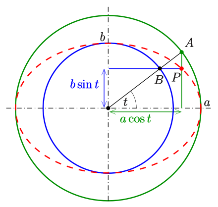
The construction of points based on the parametric equation and the interpretation of parameter t, which is due to de la Hire

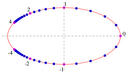
Ellipse points calculated by the rational representation with equal spaced parameters ({\displaystyle \Delta u=0.2}{\displaystyle \Delta u=0.2}).

3.1 Standard parametric representation

Using trigonometric functions, a parametric representation of the standard ellipse {\displaystyle {\tfrac {x^{2}}{a{2}}}+{\tfrac {y^{2}}{b{2}}}=1}{\tfrac {x^{2}}{a{2}}}+{\tfrac {y^{2}}{b{2}}}=1 is:

{\displaystyle (x,,y)=(a\cos t,,b\sin t),\ 0\leq t<2\pi \ .}{\displaystyle (x,,y)=(a\cos t,,b\sin t),\ 0\leq t<2\pi \ .}
The parameter t (called the eccentric anomaly in astronomy) is not the angle of {\displaystyle (x(t),y(t))}{\displaystyle (x(t),y(t))} with the x-axis, but has a geometric meaning due to Philippe de La Hire (see Drawing ellipses below).[8]

3.2 Rational representation

With the substitution {\textstyle u=\tan \left({\frac {t}{2}}\right)}{\textstyle u=\tan \left({\frac {t}{2}}\right)} and trigonometric formulae one obtains

{\displaystyle \cos t={\frac {1-u^{2}}{1+u{2}}}\ ,\quad \sin t={\frac {2u}{1+u^{2}}}}{\displaystyle \cos t={\frac {1-u^{2}}{1+u{2}}}\ ,\quad \sin t={\frac {2u}{1+u^{2}}}}
and the rational parametric equation of an ellipse

{\displaystyle {\begin{aligned}x(u)&=a{\frac {1-u^{2}}{1+u{2}}}\[10mu]y(u)&=b{\frac {2u}{1+u^{2}}}\end{aligned}};,\quad -\infty <u<\infty ;,}{\displaystyle {\begin{aligned}x(u)&=a{\frac {1-u^{2}}{1+u{2}}}\[10mu]y(u)&=b{\frac {2u}{1+u^{2}}}\end{aligned}};,\quad -\infty <u<\infty ;,}
which covers any point of the ellipse {\displaystyle {\tfrac {x^{2}}{a{2}}}+{\tfrac {y^{2}}{b{2}}}=1}{\displaystyle {\tfrac {x^{2}}{a{2}}}+{\tfrac {y^{2}}{b{2}}}=1} except the left vertex {\displaystyle (-a,,0)}{\displaystyle (-a,,0)}.

For {\displaystyle u\in [0,,1],}{\displaystyle u\in [0,,1],} this formula represents the right upper quarter of the ellipse moving counter-clockwise with increasing {\displaystyle u.}u. The left vertex is the limit {\textstyle \lim _{u\to \pm \infty }(x(u),,y(u))=(-a,,0);.}{\textstyle \lim _{u\to \pm \infty }(x(u),,y(u))=(-a,,0);.}

Alternately, if the parameter {\displaystyle [u:v]}{\displaystyle [u:v]} is considered to be a point on the real projective line {\textstyle \mathbf {P} (\mathbf {R} )}{\textstyle \mathbf {P} (\mathbf {R} )}, then the corresponding rational parametrization is

{\displaystyle [u:v]\mapsto \left(a{\frac {v^{2}-u{2}}{v^{2}+u{2}}},b{\frac {2uv}{v^{2}+u{2}}}\right).}{\displaystyle [u:v]\mapsto \left(a{\frac {v^{2}-u{2}}{v^{2}+u{2}}},b{\frac {2uv}{v^{2}+u{2}}}\right).}
Then {\textstyle [1:0]\mapsto (-a,,0).}{\textstyle [1:0]\mapsto (-a,,0).}

Rational representations of conic sections are commonly used in computer-aided design (see Bezier curve).

3.3 Tangent slope as parameter

A parametric representation, which uses the slope {\displaystyle m}m of the tangent at a point of the ellipse can be obtained from the derivative of the standard representation {\displaystyle {\vec {x}}(t)=(a\cos t,,b\sin t)^{\mathsf {T}}}{\displaystyle {\vec {x}}(t)=(a\cos t,,b\sin t)^{\mathsf {T}}}:

{\displaystyle {\vec {x}}‘(t)=(-a\sin t,,b\cos t)^{\mathsf {T}}\quad \rightarrow \quad m=-{\frac {b}{a}}\cot t\quad \rightarrow \quad \cot t=-{\frac {ma}{b}}.}{\displaystyle {\vec {x}}’(t)=(-a\sin t,,b\cos t)^{\mathsf {T}}\quad \rightarrow \quad m=-{\frac {b}{a}}\cot t\quad \rightarrow \quad \cot t=-{\frac {ma}{b}}.}
With help of trigonometric formulae one obtains:

{\displaystyle \cos t={\frac {\cot t}{\pm {\sqrt {1+\cot ^{2}t}}}}={\frac {-ma}{\pm {\sqrt {m^{2}a{2}+b^{2}}}}}\ ,\quad \quad \sin t={\frac {1}{\pm {\sqrt {1+\cot ^{2}t}}}}={\frac {b}{\pm {\sqrt {m^{2}a{2}+b^{2}}}}}.}{\displaystyle \cos t={\frac {\cot t}{\pm {\sqrt {1+\cot ^{2}t}}}}={\frac {-ma}{\pm {\sqrt {m^{2}a{2}+b^{2}}}}}\ ,\quad \quad \sin t={\frac {1}{\pm {\sqrt {1+\cot ^{2}t}}}}={\frac {b}{\pm {\sqrt {m^{2}a{2}+b^{2}}}}}.}
Replacing {\displaystyle \cos t}{\displaystyle \cos t} and {\displaystyle \sin t}\sin t of the standard representation yields:

{\displaystyle {\vec {c}}{\pm }(m)=\left(-{\frac {ma^{2}}{\pm {\sqrt {m^{2}a{2}+b^{2}}}}},;{\frac {b^{2}}{\pm {\sqrt {m^{2}a{2}+b^{2}}}}}\right),,m\in \mathbb {R} .}{\displaystyle {\vec {c}}{\pm }(m)=\left(-{\frac {ma^{2}}{\pm {\sqrt {m^{2}a{2}+b^{2}}}}},;{\frac {b^{2}}{\pm {\sqrt {m^{2}a{2}+b^{2}}}}}\right),,m\in \mathbb {R} .}
Here {\displaystyle m}m is the slope of the tangent at the corresponding ellipse point, {\displaystyle {\vec {c}}{+}}{\displaystyle {\vec {c}}{+}} is the upper and {\displaystyle {\vec {c}}{-}}{\displaystyle {\vec {c}}{-}} the lower half of the ellipse. The vertices{\displaystyle (\pm a,,0)}{\displaystyle (\pm a,,0)}, having vertical tangents, are not covered by the representation.

The equation of the tangent at point {\displaystyle {\vec {c}}{\pm }(m)}{\vec c}{\pm }(m) has the form {\displaystyle y=mx+n}{\displaystyle y=mx+n}. The still unknown {\displaystyle n}n can be determined by inserting the coordinates of the corresponding ellipse point {\displaystyle {\vec {c}}{\pm }(m)}{\vec c}{\pm }(m):

{\displaystyle y=mx\pm {\sqrt {m^{2}a{2}+b^{2}}};.}{\displaystyle y=mx\pm {\sqrt {m^{2}a{2}+b^{2}}};.}
This description of the tangents of an ellipse is an essential tool for the determination of the orthoptic of an ellipse. The orthoptic article contains another proof, without differential calculus and trigonometric formulae.

3.4 General ellipse

Another definition of an ellipse uses affine transformations:

Any ellipse is an affine image of the unit circle with equation {\displaystyle x^{2}+y{2}=1}x^2 + y^2 = 1.

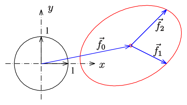
Ellipse as an affine image of the unit circle

Parametric representation
An affine transformation of the Euclidean plane has the form {\displaystyle {\vec {x}}\mapsto {\vec {f}}!{0}+A{\vec {x}}}{\displaystyle {\vec {x}}\mapsto {\vec {f}}!{0}+A{\vec {x}}}, where {\displaystyle A}A is a regular matrix (with non-zero determinant) and {\displaystyle {\vec {f}}!{0}}{\displaystyle {\vec {f}}!{0}} is an arbitrary vector. If {\displaystyle {\vec {f}}!{1},{\vec {f}}!{2}}{\displaystyle {\vec {f}}!{1},{\vec {f}}!{2}} are the column vectors of the matrix {\displaystyle A}A, the unit circle {\displaystyle (\cos(t),\sin(t))}{\displaystyle (\cos(t),\sin(t))}, {\displaystyle 0\leq t\leq 2\pi }{\displaystyle 0\leq t\leq 2\pi }, is mapped onto the ellipse:

{\displaystyle {\vec {x}}={\vec {p}}(t)={\vec {f}}!{0}+{\vec {f}}!{1}\cos t+{\vec {f}}!{2}\sin t\ .}{\displaystyle {\vec {x}}={\vec {p}}(t)={\vec {f}}!{0}+{\vec {f}}!{1}\cos t+{\vec {f}}!{2}\sin t\ .}
Here {\displaystyle {\vec {f}}!{0}}{\displaystyle {\vec {f}}!{0}} is the center and {\displaystyle {\vec {f}}!{1},;{\vec {f}}!{2}}{\displaystyle {\vec {f}}!{1},;{\vec {f}}!{2}} are the directions of two conjugate diameters, in general not perpendicular.

Vertices
The four vertices of the ellipse are {\displaystyle {\vec {p}}(t_{0}),;{\vec {p}}\left(t_{0}\pm {\tfrac {\pi }{2}}\right),;{\vec {p}}\left(t_{0}+\pi \right)}{\displaystyle {\vec {p}}(t_{0}),;{\vec {p}}\left(t_{0}\pm {\tfrac {\pi }{2}}\right),;{\vec {p}}\left(t_{0}+\pi \right)}, for a parameter {\displaystyle t=t_{0}}t=t_{0} defined by:

{\displaystyle \cot(2t_{0})={\frac {{\vec {f}}!{1}^{,2}-{\vec {f}}!{2}^{,2}}{2{\vec {f}}!{1}\cdot {\vec {f}}!{2}}}.}{\displaystyle \cot(2t_{0})={\frac {{\vec {f}}!{1}^{,2}-{\vec {f}}!{2}^{,2}}{2{\vec {f}}!{1}\cdot {\vec {f}}!{2}}}.}
(If {\displaystyle {\vec {f}}!{1}\cdot {\vec {f}}!{2}=0}{\displaystyle {\vec {f}}!{1}\cdot {\vec {f}}!{2}=0}, then {\displaystyle t_{0}=0}t_{0}=0.) This is derived as follows. The tangent vector at point {\displaystyle {\vec {p}}(t)}{\displaystyle {\vec {p}}(t)} is:

{\displaystyle {\vec {p}},‘(t)=-{\vec {f}}!{1}\sin t+{\vec {f}}!{2}\cos t\ .}{\displaystyle {\vec {p}},’(t)=-{\vec {f}}!{1}\sin t+{\vec {f}}!{2}\cos t\ .}
At a vertex parameter {\displaystyle t=t_{0}}t=t_{0}, the tangent is perpendicular to the major/minor axes, so:

{\displaystyle 0={\vec {p}}'(t)\cdot \left({\vec {p}}(t)-{\vec {f}}!{0}\right)=\left(-{\vec {f}}!{1}\sin t+{\vec {f}}!{2}\cos t\right)\cdot \left({\vec {f}}!{1}\cos t+{\vec {f}}!{2}\sin t\right).}{\displaystyle 0={\vec {p}}'(t)\cdot \left({\vec {p}}(t)-{\vec {f}}!{0}\right)=\left(-{\vec {f}}!{1}\sin t+{\vec {f}}!{2}\cos t\right)\cdot \left({\vec {f}}!{1}\cos t+{\vec {f}}!{2}\sin t\right).}
Expanding and applying the identities {\displaystyle ;\cos ^{2}t-\sin ^{2}t=\cos 2t,\ \ 2\sin t\cos t=\sin 2t;}{\displaystyle ;\cos ^{2}t-\sin ^{2}t=\cos 2t,\ \ 2\sin t\cos t=\sin 2t;} gives the equation for {\displaystyle t=t_{0};.}{\displaystyle t=t_{0};.}

Area
From Apollonios theorem (see below) one obtains:
The area of an ellipse {\displaystyle ;{\vec {x}}={\vec {f}}{0}+{\vec {f}}{1}\cos t+{\vec {f}}{2}\sin t;}{\displaystyle ;{\vec {x}}={\vec {f}}{0}+{\vec {f}}{1}\cos t+{\vec {f}}{2}\sin t;} is

{\displaystyle A=\pi |\det({\vec {f}}{1},{\vec {f}}{2})|\ .}{\displaystyle A=\pi |\det({\vec {f}}{1},{\vec {f}}{2})|\ .}
Semiaxes
With the abbreviations {\displaystyle ;M={\vec {f}}{1}^{2}+{\vec {f}}{2}^{2},\ N=\left|\det({\vec {f}}{1},{\vec {f}}{2})\right|}{\displaystyle ;M={\vec {f}}{1}^{2}+{\vec {f}}{2}^{2},\ N=\left|\det({\vec {f}}{1},{\vec {f}}{2})\right|} the statements of Apollonios’s theorem can be written as:

{\displaystyle a^{2}+b{2}=M,\quad ab=N\ .}{\displaystyle a^{2}+b{2}=M,\quad ab=N\ .}
Solving this nonlinear system for {\displaystyle a,b}a,b yields the semiaxes:

{\displaystyle a={\frac {1}{2}}({\sqrt {M+2N}}+{\sqrt {M-2N}})}{\displaystyle a={\frac {1}{2}}({\sqrt {M+2N}}+{\sqrt {M-2N}})}
{\displaystyle b={\frac {1}{2}}({\sqrt {M+2N}}-{\sqrt {M-2N}})\ .}{\displaystyle b={\frac {1}{2}}({\sqrt {M+2N}}-{\sqrt {M-2N}})\ .}
Implicit representation
Solving the parametric representation for {\displaystyle ;\cos t,\sin t;}{\displaystyle ;\cos t,\sin t;} by Cramer’s rule and using {\displaystyle ;\cos ^{2}t+\sin ^{2}t-1=0;}{\displaystyle ;\cos ^{2}t+\sin ^{2}t-1=0;}, one obtains the implicit representation

{\displaystyle \det({\vec {x}}!-!{\vec {f}}!{0},{\vec {f}}!{2})^{2}+\det({\vec {f}}!{1},{\vec {x}}!-!{\vec {f}}!{0})^{2}-\det({\vec {f}}!{1},{\vec {f}}!{2})^{2}=0}{\displaystyle \det({\vec {x}}!-!{\vec {f}}!{0},{\vec {f}}!{2})^{2}+\det({\vec {f}}!{1},{\vec {x}}!-!{\vec {f}}!{0})^{2}-\det({\vec {f}}!{1},{\vec {f}}!{2})^{2}=0}.
Conversely: If the equation

{\displaystyle x^{2}+2cxy+d{2}y^{2}-e{2}=0\ ,}{\displaystyle x^{2}+2cxy+d{2}y^{2}-e{2}=0\ ,} with {\displaystyle ;d^{2}-c{2}>0;,}{\displaystyle ;d^{2}-c{2}>0;,}
of an ellipse centered at the origin is given, then the two vectors

{\displaystyle {\vec {f}}{1}={e \choose 0},\quad {\vec {f}}{2}={\frac {e}{\sqrt {d^{2}-c{2}}}}{-c \choose 1}\ }{\displaystyle {\vec {f}}{1}={e \choose 0},\quad {\vec {f}}{2}={\frac {e}{\sqrt {d^{2}-c{2}}}}{-c \choose 1}\ }
point to two conjugate points and the tools developed above are applicable.

Example: For the ellipse with equation {\displaystyle ;x^{2}+2xy+3y{2}-1=0;}{\displaystyle ;x^{2}+2xy+3y{2}-1=0;} the vectors are

{\displaystyle {\vec {f}}{1}={1 \choose 0},\quad {\vec {f}}{2}={\frac {1}{\sqrt {2}}}{-1 \choose 1}}{\displaystyle {\vec {f}}{1}={1 \choose 0},\quad {\vec {f}}{2}={\frac {1}{\sqrt {2}}}{-1 \choose 1}}.

Rotated Standard ellipse
For {\displaystyle {\vec {f}}{0}={0 \choose 0},;{\vec {f}}{1}=a{\cos \theta \choose \sin \theta },;{\vec {f}}{2}=b{-\sin \theta \choose ;\cos \theta }}{\displaystyle {\vec {f}}{0}={0 \choose 0},;{\vec {f}}{1}=a{\cos \theta \choose \sin \theta },;{\vec {f}}{2}=b{-\sin \theta \choose ;\cos \theta }} one obtains a parametric representation of the standard ellipse rotated by angle {\displaystyle \theta }\theta :

{\displaystyle x=x_{\theta }(t)=a\cos \theta \cos t-b\sin \theta \sin t\ ,}{\displaystyle x=x_{\theta }(t)=a\cos \theta \cos t-b\sin \theta \sin t\ ,}
{\displaystyle y=y_{\theta }(t)=a\sin \theta \cos t+b\cos \theta \sin t\ .}{\displaystyle y=y_{\theta }(t)=a\sin \theta \cos t+b\cos \theta \sin t\ .}
Ellipse in space
The definition of an ellipse in this section gives a parametric representation of an arbitrary ellipse, even in space, if one allows {\displaystyle {\vec {f}}!{0},{\vec {f}}!{1},{\vec {f}}!{2}}{\displaystyle {\vec {f}}!{0},{\vec {f}}!{1},{\vec {f}}!{2}} to be vectors in space.

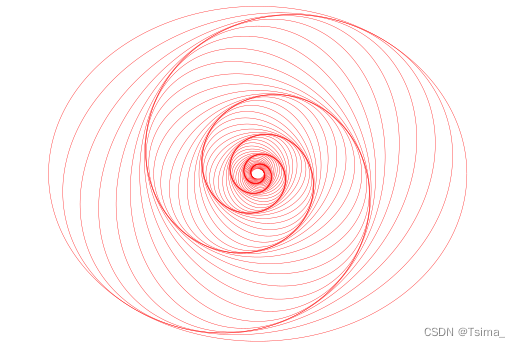
Whirls: nested, scaled and rotated ellipses. The spiral is not drawn: we see it as the locus of points where the ellipses are especially close to each other.

4 Polar forms

4.1 Polar form relative to center

In polar coordinates, with the origin at the center of the ellipse and with the angular coordinate {\displaystyle \theta }\theta measured from the major axis, the ellipse’s equation is[7]: p. 75

{\displaystyle r(\theta )={\frac {ab}{\sqrt {(b\cos \theta )^{2}+(a\sin \theta )^{2}}}}={\frac {b}{\sqrt {1-(e\cos \theta )^{2}}}}}{\displaystyle r(\theta )={\frac {ab}{\sqrt {(b\cos \theta )^{2}+(a\sin \theta )^{2}}}}={\frac {b}{\sqrt {1-(e\cos \theta )^{2}}}}}
where {\displaystyle e}e is the eccentricity, not Euler’s number

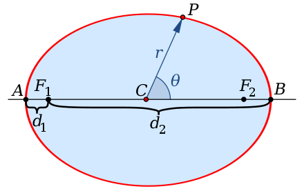
Polar coordinates centered at the center.

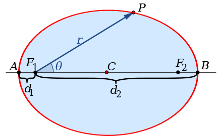
4.2 Polar form relative to focus

If instead we use polar coordinates with the origin at one focus, with the angular coordinate {\displaystyle \theta =0}\theta =0 still measured from the major axis, the ellipse’s equation is

{\displaystyle r(\theta )={\frac {a(1-e^{2})}{1\pm e\cos \theta }}}{\displaystyle r(\theta )={\frac {a(1-e^{2})}{1\pm e\cos \theta }}}
where the sign in the denominator is negative if the reference direction {\displaystyle \theta =0}\theta =0 points towards the center (as illustrated on the right), and positive if that direction points away from the center.

In the slightly more general case of an ellipse with one focus at the origin and the other focus at angular coordinate {\displaystyle \phi }\phi , the polar form is

{\displaystyle r(\theta )={\frac {a(1-e^{2})}{1-e\cos(\theta -\phi )}}.}{\displaystyle r(\theta )={\frac {a(1-e^{2})}{1-e\cos(\theta -\phi )}}.}
The angle {\displaystyle \theta }\theta in these formulas is called the true anomaly of the point. The numerator of these formulas is the semi-latus rectum {\displaystyle \ell =a(1-e^{2})}{\displaystyle \ell =a(1-e^{2})}.

Polar coordinates centered at focus.

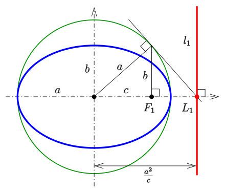
5 Eccentricity and the directrix property

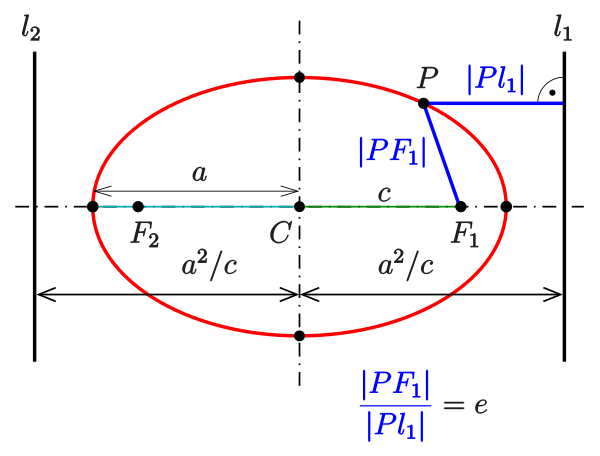
Ellipse: directrix property

Each of the two lines parallel to the minor axis, and at a distance of {\textstyle d={\frac {a^{2}}{c}}={\frac {a}{e}}}{\textstyle d={\frac {a^{2}}{c}}={\frac {a}{e}}} from it, is called a directrix of the ellipse (see diagram).

For an arbitrary point {\displaystyle P}P of the ellipse, the quotient of the distance to one focus and to the corresponding directrix (see diagram) is equal to the eccentricity:
{\displaystyle {\frac {\left|PF_{1}\right|}{\left|Pl_{1}\right|}}={\frac {\left|PF_{2}\right|}{\left|Pl_{2}\right|}}=e={\frac {c}{a}}\ .}{\displaystyle {\frac {\left|PF_{1}\right|}{\left|Pl_{1}\right|}}={\frac {\left|PF_{2}\right|}{\left|Pl_{2}\right|}}=e={\frac {c}{a}}\ .}
The proof for the pair {\displaystyle F_{1},l_{1}}{\displaystyle F_{1},l_{1}} follows from the fact that {\displaystyle \left|PF_{1}\right|^{2}=(x-c){2}+y^{{2}, \left|Pl_{1}\right|}{2}=\left(x-{\tfrac {a^{{2}}{c}}\right)}{2}}{\displaystyle \left|PF_{1}\right|^{2}=(x-c){2}+y^{{2}, \left|Pl_{1}\right|}{2}=\left(x-{\tfrac {a^{{2}}{c}}\right)}{2}} and {\displaystyle y^{2}=b{2}-{\tfrac {b^{2}}{a{2}}}x^{2}}{\displaystyle y^{2}=b{2}-{\tfrac {b^{2}}{a{2}}}x^{2}} satisfy the equation

{\displaystyle \left|PF_{1}\right|^{2}-{\frac {c^{2}}{a{2}}}\left|Pl_{1}\right|^{2}=0\ .}{\displaystyle \left|PF_{1}\right|^{2}-{\frac {c^{2}}{a{2}}}\left|Pl_{1}\right|^{2}=0\ .}
The second case is proven analogously.

The converse is also true and can be used to define an ellipse (in a manner similar to the definition of a parabola):

For any point {\displaystyle F}F (focus), any line {\displaystyle l}l (directrix) not through {\displaystyle F}F, and any real number {\displaystyle e}e with {\displaystyle 0<e<1,}{\displaystyle 0<e<1,} the ellipse is the locus of points for which the quotient of the distances to the point and to the line is {\displaystyle e,}e, that is:
{\displaystyle E=\left{P\ \left|\ {\frac {|PF|}{|Pl|}}=e\right.\right}.}{\displaystyle E=\left{P\ \left|\ {\frac {|PF|}{|Pl|}}=e\right.\right}.}
The extension to {\displaystyle e=0}e=0, which is the eccentricity of a circle, is not allowed in this context in the Euclidean plane. However, one may consider the directrix of a circle to be the line at infinity in the projective plane.

(The choice {\displaystyle e=1}e=1 yields a parabola, and if {\displaystyle e>1}e>1, a hyperbola.)

Proof
Let {\displaystyle F=(f,,0),\ e>0}{\displaystyle F=(f,,0),\ e>0}, and assume {\displaystyle (0,,0)}{\displaystyle (0,,0)} is a point on the curve. The directrix {\displaystyle l}l has equation {\displaystyle x=-{\tfrac {f}{e}}}{\displaystyle x=-{\tfrac {f}{e}}}. With {\displaystyle P=(x,,y)}{\displaystyle P=(x,,y)}, the relation {\displaystyle |PF|^{2}=e{2}|Pl|^{2}}{\displaystyle |PF|^{2}=e{2}|Pl|^{2}} produces the equations

{\displaystyle (x-f)^{2}+y{2}=e^{2}\left(x+{\frac {f}{e}}\right)^{2}=(ex+f){2}}{\displaystyle (x-f)^{2}+y{2}=e^{2}\left(x+{\frac {f}{e}}\right)^{2}=(ex+f){2}} and {\displaystyle x^{2}\left(e{2}-1\right)+2xf(1+e)-y^{2}=0.}{\displaystyle x^{2}\left(e{2}-1\right)+2xf(1+e)-y^{2}=0.}
The substitution {\displaystyle p=f(1+e)}{\displaystyle p=f(1+e)} yields

{\displaystyle x^{2}\left(e{2}-1\right)+2px-y^{2}=0.}{\displaystyle x^{2}\left(e{2}-1\right)+2px-y^{2}=0.}
This is the equation of an ellipse ({\displaystyle e<1}{\displaystyle e<1}), or a parabola ({\displaystyle e=1}e=1), or a hyperbola ({\displaystyle e>1}e>1). All of these non-degenerate conics have, in common, the origin as a vertex (see diagram).

If {\displaystyle e<1}{\displaystyle e<1}, introduce new parameters {\displaystyle a,,b}{\displaystyle a,,b} so that {\displaystyle 1-e^{2}={\tfrac {b^{2}}{a{2}}},{\text{ and }}\ p={\tfrac {b^{2}}{a}}}{\displaystyle 1-e^{2}={\tfrac {b^{2}}{a{2}}},{\text{ and }}\ p={\tfrac {b^{2}}{a}}}, and then the equation above becomes

{\displaystyle {\frac {(x-a)^{2}}{a{2}}}+{\frac {y^{2}}{b{2}}}=1\ ,}{\displaystyle {\frac {(x-a)^{2}}{a{2}}}+{\frac {y^{2}}{b{2}}}=1\ ,}
which is the equation of an ellipse with center {\displaystyle (a,,0)}{\displaystyle (a,,0)}, the x-axis as major axis, and the major/minor semi axis {\displaystyle a,,b}{\displaystyle a,,b}.

Construction of a directrix
Because of {\displaystyle c\cdot {\tfrac {a^{2}}{c}}=a{2}}{\displaystyle c\cdot {\tfrac {a^{2}}{c}}=a{2}} point {\displaystyle L_{1}}L_{1} of directrix {\displaystyle l_{1}}l_{1} (see diagram) and focus {\displaystyle F_{1}}F_{1} are inverse with respect to the circle inversion at circle {\displaystyle x^{2}+y{2}=a^{2}}{\displaystyle x^{2}+y{2}=a^{2}} (in diagram green). Hence {\displaystyle L_{1}}L_{1} can be constructed as shown in the diagram. Directrix {\displaystyle l_{1}}l_{1} is the perpendicular to the main axis at point {\displaystyle L_{1}}L_{1}.

General ellipse
If the focus is {\displaystyle F=\left(f_{1},,f_{2}\right)}{\displaystyle F=\left(f_{1},,f_{2}\right)} and the directrix {\displaystyle ux+vy+w=0}{\displaystyle ux+vy+w=0}, one obtains the equation

{\displaystyle \left(x-f_{1}\right)^{{2}+\left(y-f_{2}\right)}{2}=e^{2}{\frac {\left(ux+vy+w\right)^{2}}{u{2}+v^{2}}}\ .}{\displaystyle \left(x-f_{1}\right)^{{2}+\left(y-f_{2}\right)}{2}=e^{2}{\frac {\left(ux+vy+w\right)^{2}}{u{2}+v^{2}}}\ .}
(The right side of the equation uses the Hesse normal form of a line to calculate the distance {\displaystyle |Pl|}{\displaystyle |Pl|}.)

Pencil of conics with a common vertex and common semi-latus rectum

Construction of a directrix

6 Focus-to-focus reflection property

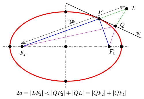
Ellipse: the tangent bisects the supplementary angle of the angle between the lines to the foci.

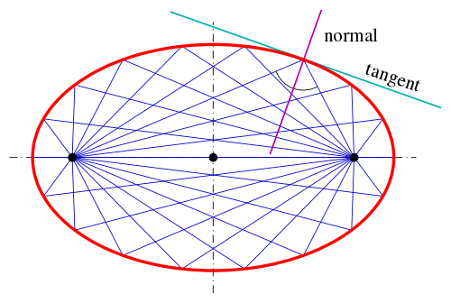
Rays from one focus reflect off the ellipse to pass through the other focus.

An ellipse possesses the following property:

The normal at a point {\displaystyle P}P bisects the angle between the lines {\displaystyle {\overline {PF_{1}}},,{\overline {PF_{2}}}}{\displaystyle {\overline {PF_{1}}},,{\overline {PF_{2}}}}.
Proof
Because the tangent is perpendicular to the normal, the statement is true for the tangent and the supplementary angle of the angle between the lines to the foci (see diagram), too.

Let {\displaystyle L}L be the point on the line {\displaystyle {\overline {PF_{2}}}}{\displaystyle {\overline {PF_{2}}}} with the distance {\displaystyle 2a}2a to the focus {\displaystyle F_{2}}F_{2}, {\displaystyle a}a is the semi-major axis of the ellipse. Let line {\displaystyle w}w be the bisector of the supplementary angle to the angle between the lines {\displaystyle {\overline {PF_{1}}},,{\overline {PF_{2}}}}{\displaystyle {\overline {PF_{1}}},,{\overline {PF_{2}}}}. In order to prove that {\displaystyle w}w is the tangent line at point {\displaystyle P}P, one checks that any point {\displaystyle Q}Q on line {\displaystyle w}w which is different from {\displaystyle P}P cannot be on the ellipse. Hence {\displaystyle w}w has only point {\displaystyle P}P in common with the ellipse and is, therefore, the tangent at point {\displaystyle P}P.

From the diagram and the triangle inequality one recognizes that {\displaystyle 2a=\left|LF_{2}\right|<\left|QF_{2}\right|+\left|QL\right|=\left|QF_{2}\right|+\left|QF_{1}\right|}{\displaystyle 2a=\left|LF_{2}\right|<\left|QF_{2}\right|+\left|QL\right|=\left|QF_{2}\right|+\left|QF_{1}\right|} holds, which means: {\displaystyle \left|QF_{2}\right|+\left|QF_{1}\right|>2a}{\displaystyle \left|QF_{2}\right|+\left|QF_{1}\right|>2a} . The equality {\displaystyle \left|QL\right|=\left|QF_{1}\right|}{\displaystyle \left|QL\right|=\left|QF_{1}\right|} is true from the Angle bisector theorem because {\displaystyle {\frac {\left|PL\right|}{\left|PF_{1}\right|}}={\frac {\left|QL\right|}{\left|QF_{1}\right|}}}{\displaystyle {\frac {\left|PL\right|}{\left|PF_{1}\right|}}={\frac {\left|QL\right|}{\left|QF_{1}\right|}}} and {\displaystyle \left|PL\right|=\left|PF_{1}\right|}{\displaystyle \left|PL\right|=\left|PF_{1}\right|} . But if {\displaystyle Q}Q is a point of the ellipse, the sum should be {\displaystyle 2a}2a.

Application
The rays from one focus are reflected by the ellipse to the second focus. This property has optical and acoustic applications similar to the reflective property of a parabola (see whispering gallery).

7 Conjugate diameters

Orthogonal diameters of a circle with a square of tangents, midpoints of parallel chords and an affine image, which is an ellipse with conjugate diameters, a parallelogram of tangents and midpoints of chords.

7.1 Definition of conjugate diameters

Main article: Conjugate diameters
A circle has the following property:

The midpoints of parallel chords lie on a diameter.
An affine transformation preserves parallelism and midpoints of line segments, so this property is true for any ellipse. (Note that the parallel chords and the diameter are no longer orthogonal.)

Definition
Two diameters {\displaystyle d_{1},,d_{2}}{\displaystyle d_{1},,d_{2}} of an ellipse are conjugate if the midpoints of chords parallel to {\displaystyle d_{1}}d_{1} lie on {\displaystyle d_{2}\ .}{\displaystyle d_{2}\ .}

From the diagram one finds:

Two diameters {\displaystyle {\overline {P_{1}Q_{1}}},,{\overline {P_{2}Q_{2}}}}{\displaystyle {\overline {P_{1}Q_{1}}},,{\overline {P_{2}Q_{2}}}} of an ellipse are conjugate whenever the tangents at {\displaystyle P_{1}}P_{1} and {\displaystyle Q_{1}}Q_{1} are parallel to {\displaystyle {\overline {P_{2}Q_{2}}}}{\displaystyle {\overline {P_{2}Q_{2}}}}.
Conjugate diameters in an ellipse generalize orthogonal diameters in a circle.

In the parametric equation for a general ellipse given above,

{\displaystyle {\vec {x}}={\vec {p}}(t)={\vec {f}}!{0}+{\vec {f}}!{1}\cos t+{\vec {f}}!{2}\sin t,}{\displaystyle {\vec {x}}={\vec {p}}(t)={\vec {f}}!{0}+{\vec {f}}!{1}\cos t+{\vec {f}}!{2}\sin t,}
any pair of points {\displaystyle {\vec {p}}(t),\ {\vec {p}}(t+\pi )}{\displaystyle {\vec {p}}(t),\ {\vec {p}}(t+\pi )} belong to a diameter, and the pair {\displaystyle {\vec {p}}\left(t+{\tfrac {\pi }{2}}\right),\ {\vec {p}}\left(t-{\tfrac {\pi }{2}}\right)}{\displaystyle {\vec {p}}\left(t+{\tfrac {\pi }{2}}\right),\ {\vec {p}}\left(t-{\tfrac {\pi }{2}}\right)} belong to its conjugate diameter.

For the common parametric representation {\displaystyle (a\cos t,b\sin t)}{\displaystyle (a\cos t,b\sin t)} of the ellipse with equation {\displaystyle {\tfrac {x^{2}}{a{2}}}+{\tfrac {y^{2}}{b{2}}}=1}{\tfrac {x^{2}}{a{2}}}+{\tfrac {y^{2}}{b{2}}}=1 one gets: The points

{\displaystyle (x_{1},y_{1})=(\pm a\cos t,\pm b\sin t)\quad }{\displaystyle (x_{1},y_{1})=(\pm a\cos t,\pm b\sin t)\quad } (signs: (+,+) or (-,-) )
{\displaystyle (x_{2},y_{2})=({\color {red}{\mp }}a\sin t,\pm b\cos t)\quad }{\displaystyle (x_{2},y_{2})=({\color {red}{\mp }}a\sin t,\pm b\cos t)\quad } (signs: (-,+) or (+,-) )
are conjugate and
{\displaystyle {\frac {x_{1}x_{2}}{a^{2}}}+{\frac {y_{1}y_{2}}{b^{2}}}=0\ .}{\displaystyle {\frac {x_{1}x_{2}}{a^{2}}}+{\frac {y_{1}y_{2}}{b^{2}}}=0\ .}
In case of a circle the last equation collapses to {\displaystyle x_{1}x_{2}+y_{1}y_{2}=0\ .}{\displaystyle x_{1}x_{2}+y_{1}y_{2}=0\ .}

7.2 Theorem of Apollonios on conjugate diameters

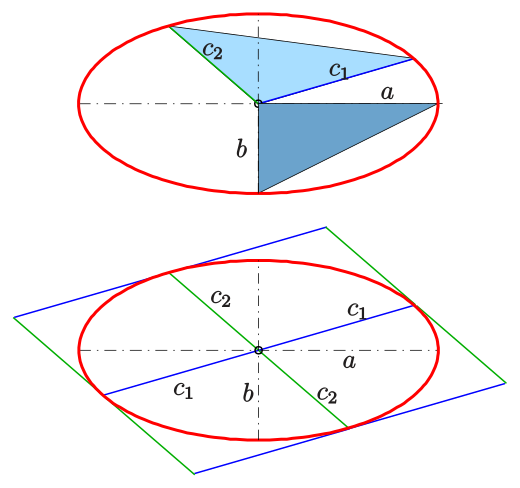
Theorem of Apollonios

For the alternative area formula

For an ellipse with semi-axes {\displaystyle a,,b}{\displaystyle a,,b} the following is true:[9][10]

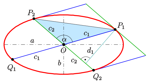
Let {\displaystyle c_{1}}{\displaystyle c_{1}} and {\displaystyle c_{2}}{\displaystyle c_{2}} be halves of two conjugate diameters (see diagram) then
{\displaystyle c_{1}^{2}+c_{2}{2}=a^{2}+b{2}}{\displaystyle c_{1}^{2}+c_{2}{2}=a^{2}+b{2}}.
The triangle {\displaystyle O,P_{1},P_{2}}{\displaystyle O,P_{1},P_{2}} with sides {\displaystyle c_{1},,c_{2}}{\displaystyle c_{1},,c_{2}} (see diagram) has the constant area {\textstyle A_{\Delta }={\frac {1}{2}}ab}{\textstyle A_{\Delta }={\frac {1}{2}}ab}, which can be expressed by {\displaystyle A_{\Delta }={\tfrac {1}{2}}c_{2}d_{1}={\tfrac {1}{2}}c_{1}c_{2}\sin \alpha }{\displaystyle A_{\Delta }={\tfrac {1}{2}}c_{2}d_{1}={\tfrac {1}{2}}c_{1}c_{2}\sin \alpha }, too. {\displaystyle d_{1}}d_{1} is the altitude of point {\displaystyle P_{1}}P_{1} and {\displaystyle \alpha }\alpha the angle between the half diameters. Hence the area of the ellipse (see section metric properties) can be written as {\displaystyle A_{el}=\pi ab=\pi c_{2}d_{1}=\pi c_{1}c_{2}\sin \alpha }{\displaystyle A_{el}=\pi ab=\pi c_{2}d_{1}=\pi c_{1}c_{2}\sin \alpha }.
The parallelogram of tangents adjacent to the given conjugate diameters has the {\displaystyle {\text{Area}}{12}=4ab\ .}{\displaystyle {\text{Area}}{12}=4ab\ .}
Proof
Let the ellipse be in the canonical form with parametric equation

{\displaystyle {\vec {p}}(t)=(a\cos t,,b\sin t)}{\displaystyle {\vec {p}}(t)=(a\cos t,,b\sin t)}.
The two points {\displaystyle {\vec {c}}{1}={\vec {p}}(t),\ {\vec {c}}{2}={\vec {p}}\left(t+{\frac {\pi }{2}}\right)}{\displaystyle {\vec {c}}{1}={\vec {p}}(t),\ {\vec {c}}{2}={\vec {p}}\left(t+{\frac {\pi }{2}}\right)} are on conjugate diameters (see previous section). From trigonometric formulae one obtains {\displaystyle {\vec {c}}{2}=(-a\sin t,,b\cos t)^{\mathsf {T}}}{\displaystyle {\vec {c}}{2}=(-a\sin t,,b\cos t)^{\mathsf {T}}} and

{\displaystyle \left|{\vec {c}}{1}\right|^{2}+\left|{\vec {c}}{2}\right|^{2}=\cdots =a^{2}+b{2}\ .}{\displaystyle \left|{\vec {c}}{1}\right|^{2}+\left|{\vec {c}}{2}\right|^{2}=\cdots =a^{2}+b{2}\ .}
The area of the triangle generated by {\displaystyle {\vec {c}}{1},,{\vec {c}}{2}}{\displaystyle {\vec {c}}{1},,{\vec {c}}{2}} is

{\displaystyle A_{\Delta }={\frac {1}{2}}\det \left({\vec {c}}{1},,{\vec {c}}{2}\right)=\cdots ={\frac {1}{2}}ab}{\displaystyle A_{\Delta }={\frac {1}{2}}\det \left({\vec {c}}{1},,{\vec {c}}{2}\right)=\cdots ={\frac {1}{2}}ab}
and from the diagram it can be seen that the area of the parallelogram is 8 times that of {\displaystyle A_{\Delta }}{\displaystyle A_{\Delta }}. Hence

{\displaystyle {\text{Area}}{12}=4ab\ .}{\displaystyle {\text{Area}}{12}=4ab\ .}

8 Orthogonal tangents

Main article: Orthoptic (geometry)
For the ellipse {\displaystyle {\tfrac {x^{2}}{a{2}}}+{\tfrac {y^{2}}{b{2}}}=1}{\tfrac {x^{2}}{a{2}}}+{\tfrac {y^{2}}{b{2}}}=1 the intersection points of orthogonal tangents lie on the circle {\displaystyle x^{2}+y{2}=a^{2}+b{2}}x^{2}+y{2}=a^{2}+b{2}.

This circle is called orthoptic or director circle of the ellipse (not to be confused with the circular directrix defined above).

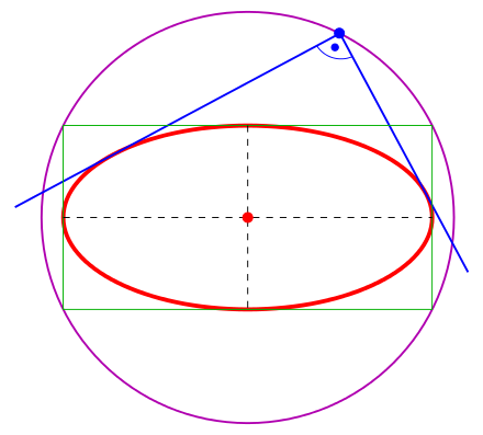
Ellipse with its orthoptic

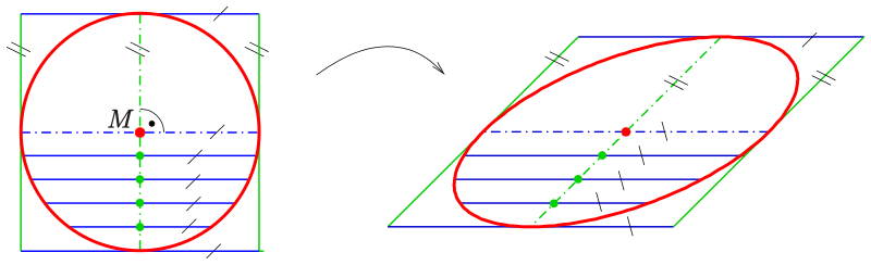
9 Drawing ellipses

Ellipses appear in descriptive geometry as images (parallel or central projection) of circles. There exist various tools to draw an ellipse. Computers provide the fastest and most accurate method for drawing an ellipse. However, technical tools (ellipsographs) to draw an ellipse without a computer exist. The principle of ellipsographs were known to Greek mathematicians such as Archimedes and Proklos.

If there is no ellipsograph available, one can draw an ellipse using an approximation by the four osculating circles at the vertices.

For any method described below, knowledge of the axes and the semi-axes is necessary (or equivalently: the foci and the semi-major axis). If this presumption is not fulfilled one has to know at least two conjugate diameters. With help of Rytz’s construction the axes and semi-axes can be retrieved.

Central projection of circles (gate)

9.1 de La Hire’s point construction

The following construction of single points of an ellipse is due to de La Hire.[11] It is based on the standard parametric representation {\displaystyle (a\cos t,,b\sin t)}{\displaystyle (a\cos t,,b\sin t)} of an ellipse:

Draw the two circles centered at the center of the ellipse with radii {\displaystyle a,b}a,b and the axes of the ellipse.
Draw a line through the center, which intersects the two circles at point {\displaystyle A}A and {\displaystyle B}B, respectively.
Draw a line through {\displaystyle A}A that is parallel to the minor axis and a line through {\displaystyle B}B that is parallel to the major axis. These lines meet at an ellipse point (see diagram).
Repeat steps (2) and (3) with different lines through the center.

de La Hire’s method

9.2 Pins-and-string method

The characterization of an ellipse as the locus of points so that sum of the distances to the foci is constant leads to a method of drawing one using two drawing pins, a length of string, and a pencil. In this method, pins are pushed into the paper at two points, which become the ellipse’s foci. A string is tied at each end to the two pins; its length after tying is {\displaystyle 2a}2a. The tip of the pencil then traces an ellipse if it is moved while keeping the string taut. Using two pegs and a rope, gardeners use this procedure to outline an elliptical flower bed—thus it is called the gardener’s ellipse.

A similar method for drawing confocal ellipses with a closed string is due to the Irish bishop Charles Graves.

Ellipse: gardener’s method

9.3 Paper strip methods

The two following methods rely on the parametric representation (see section parametric representation, above):

{\displaystyle (a\cos t,,b\sin t)}{\displaystyle (a\cos t,,b\sin t)}
This representation can be modeled technically by two simple methods. In both cases center, the axes and semi axes {\displaystyle a,,b}{\displaystyle a,,b} have to be known.

Method 1
The first method starts with

a strip of paper of length {\displaystyle a+b}a+b.
The point, where the semi axes meet is marked by {\displaystyle P}P. If the strip slides with both ends on the axes of the desired ellipse, then point {\displaystyle P}P traces the ellipse. For the proof one shows that point {\displaystyle P}P has the parametric representation {\displaystyle (a\cos t,,b\sin t)}{\displaystyle (a\cos t,,b\sin t)}, where parameter {\displaystyle t}t is the angle of the slope of the paper strip.

A technical realization of the motion of the paper strip can be achieved by a Tusi couple (see animation). The device is able to draw any ellipse with a fixed sum {\displaystyle a+b}a+b, which is the radius of the large circle. This restriction may be a disadvantage in real life. More flexible is the second paper strip method.

Ellipse construction: paper strip method 1

A variation of the paper strip method 1 uses the observation that the midpoint {\displaystyle N}N of the paper strip is moving on the circle with center {\displaystyle M}M (of the ellipse) and radius {\displaystyle {\tfrac {a+b}{2}}}{\displaystyle {\tfrac {a+b}{2}}}. Hence, the paperstrip can be cut at point {\displaystyle N}N into halves, connected again by a joint at {\displaystyle N}N and the sliding end {\displaystyle K}K fixed at the center {\displaystyle M}M (see diagram). After this operation the movement of the unchanged half of the paperstrip is unchanged.[12] This variation requires only one sliding shoe.

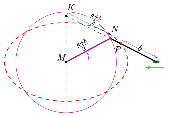
Variation of the paper strip method 1

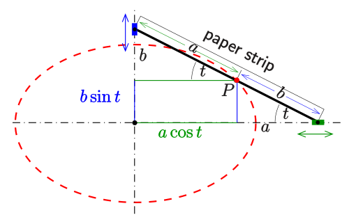
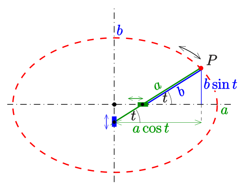
Method 2
The second method starts with

a strip of paper of length {\displaystyle a}a.
One marks the point, which divides the strip into two substrips of length {\displaystyle b}b and {\displaystyle a-b}a-b. The strip is positioned onto the axes as described in the diagram. Then the free end of the strip traces an ellipse, while the strip is moved. For the proof, one recognizes that the tracing point can be described parametrically by {\displaystyle (a\cos t,,b\sin t)}{\displaystyle (a\cos t,,b\sin t)}, where parameter {\displaystyle t}t is the angle of slope of the paper strip.

This method is the base for several ellipsographs (see section below).

Similar to the variation of the paper strip method 1 a variation of the paper strip method 2 can be established (see diagram) by cutting the part between the axes into halves.

Most ellipsograph drafting instruments are based on the second paperstrip method.

Ellipse construction: paper strip method 2

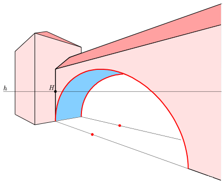
9.4 Approximation by osculating circles

From Metric properties below, one obtains:

The radius of curvature at the vertices {\displaystyle V_{1},,V_{2}}{\displaystyle V_{1},,V_{2}} is: {\displaystyle {\tfrac {b^{2}}{a}}}{\displaystyle {\tfrac {b^{2}}{a}}}
The radius of curvature at the co-vertices {\displaystyle V_{3},,V_{4}}{\displaystyle V_{3},,V_{4}} is: {\displaystyle {\tfrac {a^{2}}{b}}\ .}{\displaystyle {\tfrac {a^{2}}{b}}\ .}
The diagram shows an easy way to find the centers of curvature {\displaystyle C_{1}=\left(a-{\tfrac {b^{2}}{a}},0\right),,C_{3}=\left(0,b-{\tfrac {a^{2}}{b}}\right)}{\displaystyle C_{1}=\left(a-{\tfrac {b^{2}}{a}},0\right),,C_{3}=\left(0,b-{\tfrac {a^{2}}{b}}\right)} at vertex {\displaystyle V_{1}}V_{1} and co-vertex {\displaystyle V_{3}}V_{3}, respectively:

mark the auxiliary point {\displaystyle H=(a,,b)}{\displaystyle H=(a,,b)} and draw the line segment {\displaystyle V_{1}V_{3}\ ,}{\displaystyle V_{1}V_{3}\ ,}
draw the line through {\displaystyle H}H, which is perpendicular to the line {\displaystyle V_{1}V_{3}\ ,}{\displaystyle V_{1}V_{3}\ ,}
the intersection points of this line with the axes are the centers of the osculating circles.
(proof: simple calculation.)

The centers for the remaining vertices are found by symmetry.

With help of a French curve one draws a curve, which has smooth contact to the osculating circles.

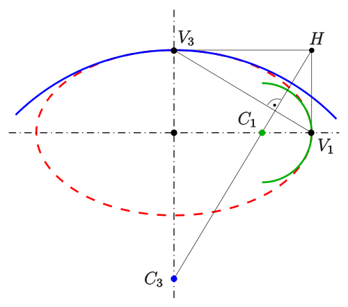
Approximation of an ellipse with osculating circles

9.5 Steiner generation

The following method to construct single points of an ellipse relies on the Steiner generation of a conic section:

Given two pencils {\displaystyle B(U),,B(V)}{\displaystyle B(U),,B(V)} of lines at two points {\displaystyle U,,V}{\displaystyle U,,V} (all lines containing {\displaystyle U}U and {\displaystyle V}V, respectively) and a projective but not perspective mapping {\displaystyle \pi }\pi of {\displaystyle B(U)}B(U) onto {\displaystyle B(V)}B(V), then the intersection points of corresponding lines form a non-degenerate projective conic section.
For the generation of points of the ellipse {\displaystyle {\tfrac {x^{2}}{a{2}}}+{\tfrac {y^{2}}{b{2}}}=1}{\displaystyle {\tfrac {x^{2}}{a{2}}}+{\tfrac {y^{2}}{b{2}}}=1} one uses the pencils at the vertices {\displaystyle V_{1},,V_{2}}{\displaystyle V_{1},,V_{2}}. Let {\displaystyle P=(0,,b)}{\displaystyle P=(0,,b)} be an upper co-vertex of the ellipse and {\displaystyle A=(-a,,2b),,B=(a,,2b)}{\displaystyle A=(-a,,2b),,B=(a,,2b)}.

{\displaystyle P}P is the center of the rectangle {\displaystyle V_{1},,V_{2},,B,,A}{\displaystyle V_{1},,V_{2},,B,,A}. The side {\displaystyle {\overline {AB}}}{\overline {AB}} of the rectangle is divided into n equal spaced line segments and this division is projected parallel with the diagonal {\displaystyle AV_{2}}{\displaystyle AV_{2}} as direction onto the line segment {\displaystyle {\overline {V_{1}B}}}{\displaystyle {\overline {V_{1}B}}} and assign the division as shown in the diagram. The parallel projection together with the reverse of the orientation is part of the projective mapping between the pencils at {\displaystyle V_{1}}V_{1} and {\displaystyle V_{2}}V_{2} needed. The intersection points of any two related lines {\displaystyle V_{1}B_{i}}{\displaystyle V_{1}B_{i}} and {\displaystyle V_{2}A_{i}}{\displaystyle V_{2}A_{i}} are points of the uniquely defined ellipse. With help of the points {\displaystyle C_{1},,\dotsc }{\displaystyle C_{1},,\dotsc } the points of the second quarter of the ellipse can be determined. Analogously one obtains the points of the lower half of the ellipse.

Steiner generation can also be defined for hyperbolas and parabolas. It is sometimes called a parallelogram method because one can use other points rather than the vertices, which starts with a parallelogram instead of a rectangle.

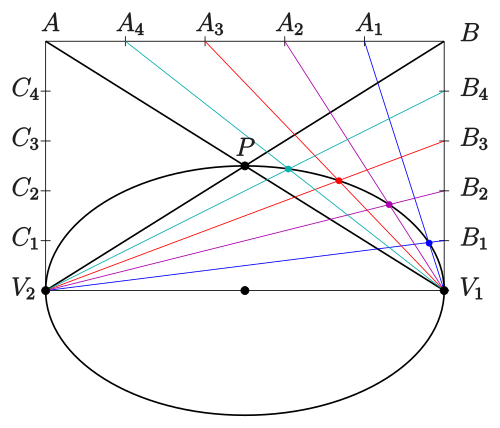
Ellipse: Steiner generation

9.6 As hypotrochoid

The ellipse is a special case of the hypotrochoid when {\displaystyle R=2r}{\displaystyle R=2r}, as shown in the adjacent image. The special case of a moving circle with radius {\displaystyle r}r inside a circle with radius {\displaystyle R=2r}{\displaystyle R=2r} is called a Tusi couple.

10 Inscribed angles and three-point form

Circle: inscribed angle theorem

10.1 Circles

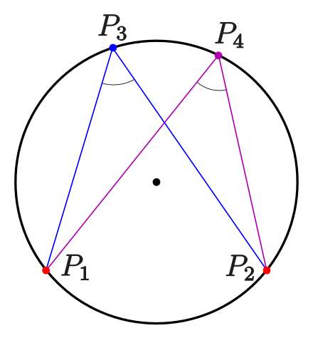
A circle with equation {\displaystyle \left(x-x_{\circ }\right)^{2}+\left(y-y_{\circ }\right)^{2}=r{2}}{\displaystyle \left(x-x_{\circ }\right)^{2}+\left(y-y_{\circ }\right)^{2}=r{2}} is uniquely determined by three points {\displaystyle \left(x_{1},y_{1}\right),;\left(x_{2},,y_{2}\right),;\left(x_{3},,y_{3}\right)}{\displaystyle \left(x_{1},y_{1}\right),;\left(x_{2},,y_{2}\right),;\left(x_{3},,y_{3}\right)} not on a line. A simple way to determine the parameters {\displaystyle x_{\circ },y_{\circ },r}{\displaystyle x_{\circ },y_{\circ },r} uses the inscribed angle theorem for circles:

For four points {\displaystyle P_{i}=\left(x_{i},,y_{i}\right),\ i=1,,2,,3,,4,,}{\displaystyle P_{i}=\left(x_{i},,y_{i}\right),\ i=1,,2,,3,,4,,} (see diagram) the following statement is true:
The four points are on a circle if and only if the angles at {\displaystyle P_{3}}P_{3} and {\displaystyle P_{4}}P_{4} are equal.
Usually one measures inscribed angles by a degree or radian θ, but here the following measurement is more convenient:

In order to measure the angle between two lines with equations {\displaystyle y=m_{1}x+d_{1},\ y=m_{2}x+d_{2},\ m_{1}\neq m_{2},}{\displaystyle y=m_{1}x+d_{1},\ y=m_{2}x+d_{2},\ m_{1}\neq m_{2},} one uses the quotient:
{\displaystyle {\frac {1+m_{1}m_{2}}{m_{2}-m_{1}}}=\cot \theta \ .}{\displaystyle {\frac {1+m_{1}m_{2}}{m_{2}-m_{1}}}=\cot \theta \ .}

10.1.1 Inscribed angle theorem for circles

For four points {\displaystyle P_{i}=\left(x_{i},,y_{i}\right),\ i=1,,2,,3,,4,,}{\displaystyle P_{i}=\left(x_{i},,y_{i}\right),\ i=1,,2,,3,,4,,} no three of them on a line, we have the following (see diagram):

The four points are on a circle, if and only if the angles at {\displaystyle P_{3}}P_{3} and {\displaystyle P_{4}}P_{4} are equal. In terms of the angle measurement above, this means:
{\displaystyle {\frac {(x_{4}-x_{1})(x_{4}-x_{2})+(y_{4}-y_{1})(y_{4}-y_{2})}{(y_{4}-y_{1})(x_{4}-x_{2})-(y_{4}-y_{2})(x_{4}-x_{1})}}={\frac {(x_{3}-x_{1})(x_{3}-x_{2})+(y_{3}-y_{1})(y_{3}-y_{2})}{(y_{3}-y_{1})(x_{3}-x_{2})-(y_{3}-y_{2})(x_{3}-x_{1})}}.}{\displaystyle {\frac {(x_{4}-x_{1})(x_{4}-x_{2})+(y_{4}-y_{1})(y_{4}-y_{2})}{(y_{4}-y_{1})(x_{4}-x_{2})-(y_{4}-y_{2})(x_{4}-x_{1})}}={\frac {(x_{3}-x_{1})(x_{3}-x_{2})+(y_{3}-y_{1})(y_{3}-y_{2})}{(y_{3}-y_{1})(x_{3}-x_{2})-(y_{3}-y_{2})(x_{3}-x_{1})}}.}
At first the measure is available only for chords not parallel to the y-axis, but the final formula works for any chord.

10.1.2 Three-point form of circle equation

As a consequence, one obtains an equation for the circle determined by three non-colinear points {\displaystyle P_{i}=\left(x_{i},,y_{i}\right)}{\displaystyle P_{i}=\left(x_{i},,y_{i}\right)}:
{\displaystyle {\frac {({\color {red}x}-x_{1})({\color {red}x}-x_{2})+({\color {red}y}-y_{1})({\color {red}y}-y_{2})}{({\color {red}y}-y_{1})({\color {red}x}-x_{2})-({\color {red}y}-y_{2})({\color {red}x}-x_{1})}}={\frac {(x_{3}-x_{1})(x_{3}-x_{2})+(y_{3}-y_{1})(y_{3}-y_{2})}{(y_{3}-y_{1})(x_{3}-x_{2})-(y_{3}-y_{2})(x_{3}-x_{1})}}.}{\displaystyle {\frac {({\color {red}x}-x_{1})({\color {red}x}-x_{2})+({\color {red}y}-y_{1})({\color {red}y}-y_{2})}{({\color {red}y}-y_{1})({\color {red}x}-x_{2})-({\color {red}y}-y_{2})({\color {red}x}-x_{1})}}={\frac {(x_{3}-x_{1})(x_{3}-x_{2})+(y_{3}-y_{1})(y_{3}-y_{2})}{(y_{3}-y_{1})(x_{3}-x_{2})-(y_{3}-y_{2})(x_{3}-x_{1})}}.}
For example, for {\displaystyle P_{1}=(2,,0),;P_{2}=(0,,1),;P_{3}=(0,,0)}{\displaystyle P_{1}=(2,,0),;P_{2}=(0,,1),;P_{3}=(0,,0)} the three-point equation is:

{\displaystyle {\frac {(x-2)x+y(y-1)}{yx-(y-1)(x-2)}}=0}{\displaystyle {\frac {(x-2)x+y(y-1)}{yx-(y-1)(x-2)}}=0}, which can be rearranged to {\displaystyle (x-1)^{2}+\left(y-{\tfrac {1}{2}}\right)^{2}={\tfrac {5}{4}}\ .}{\displaystyle (x-1)^{2}+\left(y-{\tfrac {1}{2}}\right)^{2}={\tfrac {5}{4}}\ .}
Using vectors, dot products and determinants this formula can be arranged more clearly, letting {\displaystyle {\vec {x}}=(x,,y)}{\displaystyle {\vec {x}}=(x,,y)}:

{\displaystyle {\frac {\left({\color {red}{\vec {x}}}-{\vec {x}}{1}\right)\cdot \left({\color {red}{\vec {x}}}-{\vec {x}}{2}\right)}{\det \left({\color {red}{\vec {x}}}-{\vec {x}}{1},{\color {red}{\vec {x}}}-{\vec {x}}{2}\right)}}={\frac {\left({\vec {x}}{3}-{\vec {x}}{1}\right)\cdot \left({\vec {x}}{3}-{\vec {x}}{2}\right)}{\det \left({\vec {x}}{3}-{\vec {x}}{1},{\vec {x}}{3}-{\vec {x}}{2}\right)}}.}{\displaystyle {\frac {\left({\color {red}{\vec {x}}}-{\vec {x}}{1}\right)\cdot \left({\color {red}{\vec {x}}}-{\vec {x}}{2}\right)}{\det \left({\color {red}{\vec {x}}}-{\vec {x}}{1},{\color {red}{\vec {x}}}-{\vec {x}}{2}\right)}}={\frac {\left({\vec {x}}{3}-{\vec {x}}{1}\right)\cdot \left({\vec {x}}{3}-{\vec {x}}{2}\right)}{\det \left({\vec {x}}{3}-{\vec {x}}{1},{\vec {x}}{3}-{\vec {x}}{2}\right)}}.}
The center of the circle {\displaystyle \left(x_{\circ },,y_{\circ }\right)}{\displaystyle \left(x_{\circ },,y_{\circ }\right)} satisfies:

{\displaystyle {\begin{bmatrix}1&{\frac {y_{1}-y_{2}}{x_{1}-x_{2}}}\{\frac {x_{1}-x_{3}}{y_{1}-y_{3}}}&1\end{bmatrix}}{\begin{bmatrix}x_{\circ }\y_{\circ }\end{bmatrix}}={\begin{bmatrix}{\frac {x_{1}^{2}-x_{2}{2}+y_{1}^{2}-y_{2}{2}}{2(x_{1}-x_{2})}}\{\frac {y_{1}^{2}-y_{3}{2}+x_{1}^{2}-x_{3}{2}}{2(y_{1}-y_{3})}}\end{bmatrix}}.}{\displaystyle {\begin{bmatrix}1&{\frac {y_{1}-y_{2}}{x_{1}-x_{2}}}\{\frac {x_{1}-x_{3}}{y_{1}-y_{3}}}&1\end{bmatrix}}{\begin{bmatrix}x_{\circ }\y_{\circ }\end{bmatrix}}={\begin{bmatrix}{\frac {x_{1}^{2}-x_{2}{2}+y_{1}^{2}-y_{2}{2}}{2(x_{1}-x_{2})}}\{\frac {y_{1}^{2}-y_{3}{2}+x_{1}^{2}-x_{3}{2}}{2(y_{1}-y_{3})}}\end{bmatrix}}.}
The radius is the distance between any of the three points and the center.

{\displaystyle r={\sqrt {\left(x_{1}-x_{\circ }\right)^{2}+\left(y_{1}-y_{\circ }\right)^{2}}}={\sqrt {\left(x_{2}-x_{\circ }\right)^{2}+\left(y_{2}-y_{\circ }\right)^{2}}}={\sqrt {\left(x_{3}-x_{\circ }\right)^{2}+\left(y_{3}-y_{\circ }\right)^{2}}}.}{\displaystyle r={\sqrt {\left(x_{1}-x_{\circ }\right)^{2}+\left(y_{1}-y_{\circ }\right)^{2}}}={\sqrt {\left(x_{2}-x_{\circ }\right)^{2}+\left(y_{2}-y_{\circ }\right)^{2}}}={\sqrt {\left(x_{3}-x_{\circ }\right)^{2}+\left(y_{3}-y_{\circ }\right)^{2}}}.}

10.2 Ellipses

This section, we consider the family of ellipses defined by equations {\displaystyle {\tfrac {\left(x-x_{\circ }\right)^{2}}{a{2}}}+{\tfrac {\left(y-y_{\circ }\right)^{2}}{b{2}}}=1}{\displaystyle {\tfrac {\left(x-x_{\circ }\right)^{2}}{a{2}}}+{\tfrac {\left(y-y_{\circ }\right)^{2}}{b{2}}}=1} with a fixed eccentricity {\displaystyle e}e. It is convenient to use the parameter:

{\displaystyle {\color {blue}q}={\frac {a^{2}}{b{2}}}={\frac {1}{1-e^{2}}},}{\displaystyle {\color {blue}q}={\frac {a^{2}}{b{2}}}={\frac {1}{1-e^{2}}},}
and to write the ellipse equation as:

{\displaystyle \left(x-x_{\circ }\right)^{2}+{\color {blue}q},\left(y-y_{\circ }\right)^{2}=a{2},}{\displaystyle \left(x-x_{\circ }\right)^{2}+{\color {blue}q},\left(y-y_{\circ }\right)^{2}=a{2},}
where q is fixed and {\displaystyle x_{\circ },,y_{\circ },,a}{\displaystyle x_{\circ },,y_{\circ },,a} vary over the real numbers. (Such ellipses have their axes parallel to the coordinate axes: if {\displaystyle q<1}{\displaystyle q<1}, the major axis is parallel to the x-axis; if {\displaystyle q>1}{\displaystyle q>1}, it is parallel to the y-axis.)

Like a circle, such an ellipse is determined by three points not on a line.

For this family of ellipses, one introduces the following q-analog angle measure, which is not a function of the usual angle measure θ:[13][14]

In order to measure an angle between two lines with equations {\displaystyle y=m_{1}x+d_{1},\ y=m_{2}x+d_{2},\ m_{1}\neq m_{2}}{\displaystyle y=m_{1}x+d_{1},\ y=m_{2}x+d_{2},\ m_{1}\neq m_{2}} one uses the quotient:
{\displaystyle {\frac {1+{\color {blue}q};m_{1}m_{2}}{m_{2}-m_{1}}}\ .}{\displaystyle {\frac {1+{\color {blue}q};m_{1}m_{2}}{m_{2}-m_{1}}}\ .}

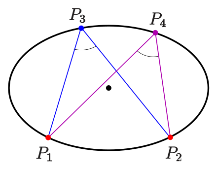
Inscribed angle theorem for an ellipse

10.2.1 Inscribed angle theorem for ellipses

Given four points {\displaystyle P_{i}=\left(x_{i},,y_{i}\right),\ i=1,,2,,3,,4}{\displaystyle P_{i}=\left(x_{i},,y_{i}\right),\ i=1,,2,,3,,4}, no three of them on a line (see diagram).
The four points are on an ellipse with equation {\displaystyle (x-x_{\circ })^{2}+{\color {blue}q},(y-y_{\circ })^{2}=a{2}}{\displaystyle (x-x_{\circ })^{2}+{\color {blue}q},(y-y_{\circ })^{2}=a{2}} if and only if the angles at {\displaystyle P_{3}}P_{3} and {\displaystyle P_{4}}P_{4} are equal in the sense of the measurement above—that is, if
{\displaystyle {\frac {(x_{4}-x_{1})(x_{4}-x_{2})+{\color {blue}q};(y_{4}-y_{1})(y_{4}-y_{2})}{(y_{4}-y_{1})(x_{4}-x_{2})-(y_{4}-y_{2})(x_{4}-x_{1})}}={\frac {(x_{3}-x_{1})(x_{3}-x_{2})+{\color {blue}q};(y_{3}-y_{1})(y_{3}-y_{2})}{(y_{3}-y_{1})(x_{3}-x_{2})-(y_{3}-y_{2})(x_{3}-x_{1})}}\ .}{\displaystyle {\frac {(x_{4}-x_{1})(x_{4}-x_{2})+{\color {blue}q};(y_{4}-y_{1})(y_{4}-y_{2})}{(y_{4}-y_{1})(x_{4}-x_{2})-(y_{4}-y_{2})(x_{4}-x_{1})}}={\frac {(x_{3}-x_{1})(x_{3}-x_{2})+{\color {blue}q};(y_{3}-y_{1})(y_{3}-y_{2})}{(y_{3}-y_{1})(x_{3}-x_{2})-(y_{3}-y_{2})(x_{3}-x_{1})}}\ .}
At first the measure is available only for chords which are not parallel to the y-axis. But the final formula works for any chord. The proof follows from a straightforward calculation. For the direction of proof given that the points are on an ellipse, one can assume that the center of the ellipse is the origin.

10.2.2 Three-point form of ellipse equation

A consequence, one obtains an equation for the ellipse determined by three non-colinear points {\displaystyle P_{i}=\left(x_{i},,y_{i}\right)}{\displaystyle P_{i}=\left(x_{i},,y_{i}\right)}:
{\displaystyle {\frac {({\color {red}x}-x_{1})({\color {red}x}-x_{2})+{\color {blue}q}😭{\color {red}y}-y_{1})({\color {red}y}-y_{2})}{({\color {red}y}-y_{1})({\color {red}x}-x_{2})-({\color {red}y}-y_{2})({\color {red}x}-x_{1})}}={\frac {(x_{3}-x_{1})(x_{3}-x_{2})+{\color {blue}q};(y_{3}-y_{1})(y_{3}-y_{2})}{(y_{3}-y_{1})(x_{3}-x_{2})-(y_{3}-y_{2})(x_{3}-x_{1})}}\ .}{\displaystyle {\frac {({\color {red}x}-x_{1})({\color {red}x}-x_{2})+{\color {blue}q}😭{\color {red}y}-y_{1})({\color {red}y}-y_{2})}{({\color {red}y}-y_{1})({\color {red}x}-x_{2})-({\color {red}y}-y_{2})({\color {red}x}-x_{1})}}={\frac {(x_{3}-x_{1})(x_{3}-x_{2})+{\color {blue}q};(y_{3}-y_{1})(y_{3}-y_{2})}{(y_{3}-y_{1})(x_{3}-x_{2})-(y_{3}-y_{2})(x_{3}-x_{1})}}\ .}
For example, for {\displaystyle P_{1}=(2,,0),;P_{2}=(0,,1),;P_{3}=(0,,0)}{\displaystyle P_{1}=(2,,0),;P_{2}=(0,,1),;P_{3}=(0,,0)} and {\displaystyle q=4}q=4 one obtains the three-point form

{\displaystyle {\frac {(x-2)x+4y(y-1)}{yx-(y-1)(x-2)}}=0}{\displaystyle {\frac {(x-2)x+4y(y-1)}{yx-(y-1)(x-2)}}=0} and after conversion {\displaystyle {\frac {(x-1)^{2}}{2}}+{\frac {\left(y-{\frac {1}{2}}\right)^{2}}{\frac {1}{2}}}=1.}{\displaystyle {\frac {(x-1)^{2}}{2}}+{\frac {\left(y-{\frac {1}{2}}\right)^{2}}{\frac {1}{2}}}=1.}
Analogously to the circle case, the equation can be written more clearly using vectors:

{\displaystyle {\frac {\left({\color {red}{\vec {x}}}-{\vec {x}}{1}\right)*\left({\color {red}{\vec {x}}}-{\vec {x}}{2}\right)}{\det \left({\color {red}{\vec {x}}}-{\vec {x}}{1},{\color {red}{\vec {x}}}-{\vec {x}}{2}\right)}}={\frac {\left({\vec {x}}{3}-{\vec {x}}{1}\right)\left({\vec {x}}{3}-{\vec {x}}{2}\right)}{\det \left({\vec {x}}{3}-{\vec {x}}{1},{\vec {x}}{3}-{\vec {x}}{2}\right)}},}{\displaystyle {\frac {\left({\color {red}{\vec {x}}}-{\vec {x}}_{1}\right)\left({\color {red}{\vec {x}}}-{\vec {x}}{2}\right)}{\det \left({\color {red}{\vec {x}}}-{\vec {x}}{1},{\color {red}{\vec {x}}}-{\vec {x}}{2}\right)}}={\frac {\left({\vec {x}}{3}-{\vec {x}}{1}\right)*\left({\vec {x}}{3}-{\vec {x}}{2}\right)}{\det \left({\vec {x}}{3}-{\vec {x}}{1},{\vec {x}}{3}-{\vec {x}}{2}\right)}},}
where {\displaystyle } is the modified dot product {\displaystyle {\vec {u}}*{\vec {v}}=u{x}v_{x}+{\color {blue}q},u_{y}v_{y}.}{\displaystyle {\vec {u}}*{\vec {v}}=u_{x}v_{x}+{\color {blue}q},u_{y}v_{y}.}

11 Pole-polar relation

Any ellipse can be described in a suitable coordinate system by an equation {\displaystyle {\tfrac {x^{2}}{a{2}}}+{\tfrac {y^{2}}{b{2}}}=1}{\displaystyle {\tfrac {x^{2}}{a{2}}}+{\tfrac {y^{2}}{b{2}}}=1}. The equation of the tangent at a point {\displaystyle P_{1}=\left(x_{1},,y_{1}\right)}{\displaystyle P_{1}=\left(x_{1},,y_{1}\right)} of the ellipse is {\displaystyle {\tfrac {x_{1}x}{a^{2}}}+{\tfrac {y_{1}y}{b^{2}}}=1.}{\displaystyle {\tfrac {x_{1}x}{a^{2}}}+{\tfrac {y_{1}y}{b^{2}}}=1.} If one allows point {\displaystyle P_{1}=\left(x_{1},,y_{1}\right)}{\displaystyle P_{1}=\left(x_{1},,y_{1}\right)} to be an arbitrary point different from the origin, then

point {\displaystyle P_{1}=\left(x_{1},,y_{1}\right)\neq (0,,0)}{\displaystyle P_{1}=\left(x_{1},,y_{1}\right)\neq (0,,0)} is mapped onto the line {\displaystyle {\tfrac {x_{1}x}{a^{2}}}+{\tfrac {y_{1}y}{b^{2}}}=1}{\displaystyle {\tfrac {x_{1}x}{a^{2}}}+{\tfrac {y_{1}y}{b^{2}}}=1}, not through the center of the ellipse.
This relation between points and lines is a bijection.

The inverse function maps

line {\displaystyle y=mx+d,\ d\neq 0}{\displaystyle y=mx+d,\ d\neq 0} onto the point {\displaystyle \left(-{\tfrac {ma^{2}}{d}},,{\tfrac {b^{2}}{d}}\right)}{\displaystyle \left(-{\tfrac {ma^{2}}{d}},,{\tfrac {b^{2}}{d}}\right)} and
line {\displaystyle x=c,\ c\neq 0}{\displaystyle x=c,\ c\neq 0} onto the point {\displaystyle \left({\tfrac {a^{2}}{c}},,0\right).}{\displaystyle \left({\tfrac {a^{2}}{c}},,0\right).}
Such a relation between points and lines generated by a conic is called pole-polar relation or polarity. The pole is the point; the polar the line.

By calculation one can confirm the following properties of the pole-polar relation of the ellipse:

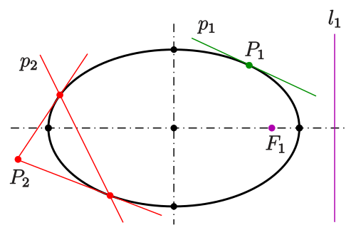
For a point (pole) on the ellipse, the polar is the tangent at this point (see diagram: {\displaystyle P_{1},,p_{1}}{\displaystyle P_{1},,p_{1}}).
For a pole {\displaystyle P}P outside the ellipse, the intersection points of its polar with the ellipse are the tangency points of the two tangents passing {\displaystyle P}P (see diagram: {\displaystyle P_{2},,p_{2}}{\displaystyle P_{2},,p_{2}}).
For a point within the ellipse, the polar has no point with the ellipse in common (see diagram: {\displaystyle F_{1},,l_{1}}{\displaystyle F_{1},,l_{1}}).
The intersection point of two polars is the pole of the line through their poles.
The foci {\displaystyle (c,,0)}{\displaystyle (c,,0)} and {\displaystyle (-c,,0)}{\displaystyle (-c,,0)}, respectively, and the directrices {\displaystyle x={\tfrac {a^{2}}{c}}}{\displaystyle x={\tfrac {a^{2}}{c}}} and {\displaystyle x=-{\tfrac {a^{2}}{c}}}{\displaystyle x=-{\tfrac {a^{2}}{c}}}, respectively, belong to pairs of pole and polar. Because they are even polar pairs with respect to the circle {\displaystyle x^{2}+y{2}=a^{2}}{\displaystyle x^{2}+y{2}=a^{2}}, the directrices can be constructed by compass and straightedge (see Inversive geometry).
Pole-polar relations exist for hyperbolas and parabolas as well.

Ellipse: pole-polar relation

12 Metric properties

All metric properties given below refer to an ellipse with equation

{\displaystyle {\frac {x^{2}}{a{2}}}+{\frac {y^{2}}{b{2}}}=1}{\displaystyle {\frac {x^{2}}{a{2}}}+{\frac {y^{2}}{b{2}}}=1}

(1)

except for the section on the area enclosed by a tilted ellipse, where the generalized form of Eq.(1) will be given.

12.1 Area

The area {\displaystyle A_{\text{ellipse}}}A_{\text{ellipse}} enclosed by an ellipse is:

{\displaystyle A_{\text{ellipse}}=\pi ab}{\displaystyle A_{\text{ellipse}}=\pi ab}

(2)

where {\displaystyle a}a and {\displaystyle b}b are the lengths of the semi-major and semi-minor axes, respectively. The area formula {\displaystyle \pi ab}{\displaystyle \pi ab} is intuitive: start with a circle of radius {\displaystyle b}b (so its area is {\displaystyle \pi b^{2}}{\displaystyle \pi b^{2}}) and stretch it by a factor {\displaystyle a/b}a/b to make an ellipse. This scales the area by the same factor: {\displaystyle \pi b^{2}(a/b)=\pi ab.}{\displaystyle \pi b^{2}(a/b)=\pi ab.}[15] However, using the same approach for the circumference would be fallacious – compare the integrals {\textstyle \int f(x),dx}{\textstyle \int f(x),dx} and {\textstyle \int {\sqrt {1+f’^{2}(x)}},dx}{\textstyle \int {\sqrt {1+f’^{2}(x)}},dx}. It is also easy to rigorously prove the area formula using integration as follows. Equation (1) can be rewritten as {\textstyle y(x)=b{\sqrt {1-x^{2}/a{2}}}.}{\textstyle y(x)=b{\sqrt {1-x^{2}/a{2}}}.} For {\displaystyle x\in [-a,a],}{\displaystyle x\in [-a,a],} this curve is the top half of the ellipse. So twice the integral of {\displaystyle y(x)}y(x) over the interval {\displaystyle [-a,a]}[-a,a] will be the area of the ellipse:

{\displaystyle {\begin{aligned}A_{\text{ellipse}}&=\int _{-a}^{a}2b{\sqrt {1-{\frac {x^{2}}{a{2}}}}},dx\&={\frac {b}{a}}\int {-a}^{a}2{\sqrt {a^{2}-x{2}}},dx.\end{aligned}}}{\displaystyle {\begin{aligned}A{\text{ellipse}}&=\int _{-a}^{a}2b{\sqrt {1-{\frac {x^{2}}{a{2}}}}},dx\&={\frac {b}{a}}\int _{-a}^{a}2{\sqrt {a^{2}-x{2}}},dx.\end{aligned}}}
The second integral is the area of a circle of radius {\displaystyle a,}a, that is, {\displaystyle \pi a^{2}.}{\displaystyle \pi a^{2}.} So

{\displaystyle A_{\text{ellipse}}={\frac {b}{a}}\pi a^{2}=\pi ab.}{\displaystyle A_{\text{ellipse}}={\frac {b}{a}}\pi a^{2}=\pi ab.}
An ellipse defined implicitly by {\displaystyle Ax^{2}+Bxy+Cy{2}=1}{\displaystyle Ax^{2}+Bxy+Cy{2}=1} has area {\displaystyle 2\pi /{\sqrt {4AC-B^{2}}}.}{\displaystyle 2\pi /{\sqrt {4AC-B^{2}}}.}

The area can also be expressed in terms of eccentricity and the length of the semi-major axis as {\displaystyle a^{2}\pi {\sqrt {1-e^{2}}}}{\displaystyle a^{2}\pi {\sqrt {1-e^{2}}}} (obtained by solving for flattening, then computing the semi-minor axis).

So far we have dealt with erect ellipses, whose major and minor axes are parallel to the {\displaystyle x}x and {\displaystyle y}y axes. However, some applications require tilted ellipses. In charged-particle beam optics, for instance, the enclosed area of an erect or tilted ellipse is an important property of the beam, its emittance. In this case a simple formula still applies, namely

{\displaystyle A_{\text{ellipse}}=\pi ;y_{\text{int}},x_{\text{max}}=\pi ;x_{\text{int}},y_{\text{max}}}{\displaystyle A_{\text{ellipse}}=\pi ;y_{\text{int}},x_{\text{max}}=\pi ;x_{\text{int}},y_{\text{max}}}

(3)

where {\displaystyle y_{\text{int}}}{\displaystyle y_{\text{int}}}, {\displaystyle x_{\text{int}}}{\displaystyle x_{\text{int}}} are intercepts and {\displaystyle x_{\text{max}}}{\displaystyle x_{\text{max}}}, {\displaystyle y_{\text{max}}}{\displaystyle y_{\text{max}}} are maximum values. It follows directly from Apollonios’s theorem.

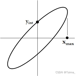
The area enclosed by a tilted ellipse is {\displaystyle \pi ;y_{\text{int}},x_{\text{max}}}{\displaystyle \pi ;y_{\text{int}},x_{\text{max}}}.

12.2 Circumference

Further information: Quarter meridian

The circumference {\displaystyle C}C of an ellipse is:

{\displaystyle C,=,4a\int _{0}^{\pi /2}{\sqrt {1-e^{2}\sin ^{2}\theta }}\ d\theta ,=,4a,E(e)}{\displaystyle C,=,4a\int _{0}^{\pi /2}{\sqrt {1-e^{2}\sin ^{2}\theta }}\ d\theta ,=,4a,E(e)}
where again {\displaystyle a}a is the length of the semi-major axis, {\textstyle e={\sqrt {1-b^{2}/a{2}}}}{\textstyle e={\sqrt {1-b^{2}/a{2}}}} is the eccentricity, and the function {\displaystyle E}E is the complete elliptic integral of the second kind,

{\displaystyle E(e),=,\int _{0}^{\pi /2}{\sqrt {1-e^{2}\sin ^{2}\theta }}\ d\theta }{\displaystyle E(e),=,\int _{0}^{\pi /2}{\sqrt {1-e^{2}\sin ^{2}\theta }}\ d\theta }
which is in general not an elementary function.

The circumference of the ellipse may be evaluated in terms of {\displaystyle E(e)}E(e) using Gauss’s arithmetic-geometric mean;[16] this is a quadratically converging iterative method (see here for details).

The exact infinite series is:

{\displaystyle {\begin{aligned}C&=2\pi a\left[{1-\left({\frac {1}{2}}\right)^{2}e{2}-\left({\frac {1\cdot 3}{2\cdot 4}}\right)^{2}{\frac {e^{4}}{3}}-\left({\frac {1\cdot 3\cdot 5}{2\cdot 4\cdot 6}}\right)^{2}{\frac {e^{6}}{5}}-\cdots }\right]\&=2\pi a\left[1-\sum _{n=1}^{\infty }\left({\frac {(2n-1)!!}{(2n)!!}}\right)^{2}{\frac {e^{2n}}{2n-1}}\right]\&=-2\pi a\sum _{n=0}^{\infty }\left({\frac {(2n-1)!!}{(2n)!!}}\right)^{2}{\frac {e^{2n}}{2n-1}},\end{aligned}}}{\displaystyle {\begin{aligned}C&=2\pi a\left[{1-\left({\frac {1}{2}}\right)^{2}e{2}-\left({\frac {1\cdot 3}{2\cdot 4}}\right)^{2}{\frac {e^{4}}{3}}-\left({\frac {1\cdot 3\cdot 5}{2\cdot 4\cdot 6}}\right)^{2}{\frac {e^{6}}{5}}-\cdots }\right]\&=2\pi a\left[1-\sum _{n=1}^{\infty }\left({\frac {(2n-1)!!}{(2n)!!}}\right)^{2}{\frac {e^{2n}}{2n-1}}\right]\&=-2\pi a\sum _{n=0}^{\infty }\left({\frac {(2n-1)!!}{(2n)!!}}\right)^{2}{\frac {e^{2n}}{2n-1}},\end{aligned}}}
where {\displaystyle n!!}n!! is the double factorial (extended to negative odd integers by the recurrence relation {\displaystyle (2n-1)!!=(2n+1)!!/(2n+1)}{\displaystyle (2n-1)!!=(2n+1)!!/(2n+1)}, for {\displaystyle n\leq 0}{\displaystyle n\leq 0}). This series converges, but by expanding in terms of {\displaystyle h=(a-b)^{2}/(a+b){2},}{\displaystyle h=(a-b)^{2}/(a+b){2},} James Ivory[17] and Bessel[18] derived an expression that converges much more rapidly:

{\displaystyle {\begin{aligned}C&=\pi (a+b)\sum _{n=0}^{\infty }\left({\frac {(2n-3)!!}{2^{{n}n!}}\right)}{2}h^{n}\&=\pi (a+b)\left[1+{\frac {h}{4}}+\sum _{n=2}^{\infty }\left({\frac {(2n-3)!!}{2^{{n}n!}}\right)}{2}h^{n}\right]\&=\pi (a+b)\left[1+\sum _{n=1}^{\infty }\left({\frac {(2n-1)!!}{2^{{n}n!}}\right)}{2}{\frac {h^{n}}{(2n-1){2}}}\right].\end{aligned}}}{\displaystyle {\begin{aligned}C&=\pi (a+b)\sum _{n=0}^{\infty }\left({\frac {(2n-3)!!}{2^{{n}n!}}\right)}{2}h^{n}\&=\pi (a+b)\left[1+{\frac {h}{4}}+\sum _{n=2}^{\infty }\left({\frac {(2n-3)!!}{2^{{n}n!}}\right)}{2}h^{n}\right]\&=\pi (a+b)\left[1+\sum _{n=1}^{\infty }\left({\frac {(2n-1)!!}{2^{{n}n!}}\right)}{2}{\frac {h^{n}}{(2n-1){2}}}\right].\end{aligned}}}
Srinivasa Ramanujan gave two close approximations for the circumference in §16 of "Modular Equations and Approximations to {\displaystyle \pi }\pi ";[19] they are

{\displaystyle C\approx \pi {\biggl [}3(a+b)-{\sqrt {(3a+b)(a+3b)}}{\biggr ]}=\pi {\biggl [}3(a+b)-{\sqrt {10ab+3\left(a^{2}+b{2}\right)}}{\biggr ]}}{\displaystyle C\approx \pi {\biggl [}3(a+b)-{\sqrt {(3a+b)(a+3b)}}{\biggr ]}=\pi {\biggl [}3(a+b)-{\sqrt {10ab+3\left(a^{2}+b{2}\right)}}{\biggr ]}}
and

{\displaystyle C\approx \pi \left(a+b\right)\left(1+{\frac {3h}{10+{\sqrt {4-3h}}}}\right),}{\displaystyle C\approx \pi \left(a+b\right)\left(1+{\frac {3h}{10+{\sqrt {4-3h}}}}\right),}
where {\displaystyle h}h takes on the same meaning as above. The errors in these approximations, which were obtained empirically, are of order {\displaystyle h^{3}}h{3} and {\displaystyle h^{5},}{\displaystyle h^{5},} respectively.

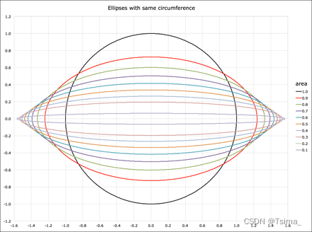
Ellipses with same circumference

12.3 Arc length

Further information: Meridian arc § Calculation
More generally, the arc length of a portion of the circumference, as a function of the angle subtended (or x-coordinates of any two points on the upper half of the ellipse), is given by an incomplete elliptic integral. The upper half of an ellipse is parameterized by

{\displaystyle y=b{\sqrt {1-{\frac {x^{2}}{a{2}}}}}.}{\displaystyle y=b{\sqrt {1-{\frac {x^{2}}{a{2}}}}}.}
Then the arc length {\displaystyle s}s from {\displaystyle x_{1}}x_{1} to {\displaystyle x_{2}}x_{2} is:

{\displaystyle s=-b\int {\arccos {\frac {x{1}}{a}}}^{\arccos {\frac {x_{2}}{a}}}{\sqrt {1-\left(1-{\frac {a^{2}}{b{2}}}\right)\sin ^{2}z}},dz.}{\displaystyle s=-b\int {\arccos {\frac {x{1}}{a}}}^{\arccos {\frac {x_{2}}{a}}}{\sqrt {1-\left(1-{\frac {a^{2}}{b{2}}}\right)\sin ^{2}z}},dz.}
This is equivalent to

{\displaystyle s=b\left[E\left(z;{\Biggl |};1-{\frac {a^{2}}{b{2}}}\right)\right]{\arccos {\frac {x{2}}{a}}}^{\arccos {\frac {x_{1}}{a}}}}{\displaystyle s=b\left[E\left(z;{\Biggl |};1-{\frac {a^{2}}{b{2}}}\right)\right]{\arccos {\frac {x{2}}{a}}}^{\arccos {\frac {x_{1}}{a}}}}
where {\displaystyle E(z\mid m)}{\displaystyle E(z\mid m)} is the incomplete elliptic integral of the second kind with parameter {\displaystyle m=k^{2}.}{\displaystyle m=k^{2}.}

Some lower and upper bounds on the circumference of the canonical ellipse {\displaystyle x^{2}/a{2}+y^{2}/b{2}=1}x^{2}/a{2}+y^{2}/b{2}=1 with {\displaystyle a\geq b}a\geq b are[20]

{\displaystyle {\begin{aligned}2\pi b&\leq C\leq 2\pi a,\\pi (a+b)&\leq C\leq 4(a+b),\4{\sqrt {a^{2}+b{2}}}&\leq C\leq {\sqrt {2}}\pi {\sqrt {a^{2}+b{2}}}.\end{aligned}}}{\displaystyle {\begin{aligned}2\pi b&\leq C\leq 2\pi a,\\pi (a+b)&\leq C\leq 4(a+b),\4{\sqrt {a^{2}+b{2}}}&\leq C\leq {\sqrt {2}}\pi {\sqrt {a^{2}+b{2}}}.\end{aligned}}}
Here the upper bound {\displaystyle 2\pi a}2\pi a is the circumference of a circumscribed concentric circle passing through the endpoints of the ellipse’s major axis, and the lower bound {\displaystyle 4{\sqrt {a^{2}+b{2}}}}4{\sqrt {a^{2}+b{2}}} is the perimeter of an inscribed rhombus with vertices at the endpoints of the major and the minor axes.

12.4 Curvature

The curvature is given by {\displaystyle \kappa ={\frac {1}{a^{2}b{2}}}\left({\frac {x^{2}}{a{4}}}+{\frac {y^{2}}{b{4}}}\right)^{-{\frac {3}{2}}}\ ,}{\displaystyle \kappa ={\frac {1}{a^{2}b{2}}}\left({\frac {x^{2}}{a{4}}}+{\frac {y^{2}}{b{4}}}\right)^{-{\frac {3}{2}}}\ ,} radius of curvature at point {\displaystyle (x,y)}(x,y):

{\displaystyle \rho =a^{2}b{2}\left({\frac {x^{2}}{a{4}}}+{\frac {y^{2}}{b{4}}}\right)^{\frac {3}{2}}={\frac {1}{a^{4}b{4}}}{\sqrt {\left(a^{4}y{2}+b^{4}x{2}\right)^{3}}}\ .}{\displaystyle \rho =a^{2}b{2}\left({\frac {x^{2}}{a{4}}}+{\frac {y^{2}}{b{4}}}\right)^{\frac {3}{2}}={\frac {1}{a^{4}b{4}}}{\sqrt {\left(a^{4}y{2}+b^{4}x{2}\right)^{3}}}\ .}
Radius of curvature at the two vertices {\displaystyle (\pm a,0)}(\pm a,0) and the centers of curvature:

{\displaystyle \rho _{0}={\frac {b^{2}}{a}}=p\ ,\qquad \left(\pm {\frac {c^{2}}{a}},{\bigg |},0\right)\ .}{\displaystyle \rho _{0}={\frac {b^{2}}{a}}=p\ ,\qquad \left(\pm {\frac {c^{2}}{a}},{\bigg |},0\right)\ .}
Radius of curvature at the two co-vertices {\displaystyle (0,\pm b)}{\displaystyle (0,\pm b)} and the centers of curvature:

{\displaystyle \rho _{1}={\frac {a^{2}}{b}}\ ,\qquad \left(0,{\bigg |},\pm {\frac {c^{2}}{b}}\right)\ .}{\displaystyle \rho _{1}={\frac {a^{2}}{b}}\ ,\qquad \left(0,{\bigg |},\pm {\frac {c^{2}}{b}}\right)\ .}

13 In triangle geometry

Ellipses appear in triangle geometry as

Steiner ellipse: ellipse through the vertices of the triangle with center at the centroid,
inellipses: ellipses which touch the sides of a triangle. Special cases are the Steiner inellipse and the Mandart inellipse.

14 As plane sections of quadrics

Ellipses appear as plane sections of the following quadrics:

Ellipsoid
Elliptic cone
Elliptic cylinder
Hyperboloid of one sheet
Hyperboloid of two sheets

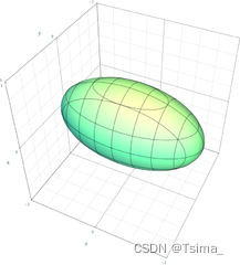
Ellipsoid

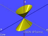
Elliptic cone

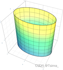
Elliptic cylinder

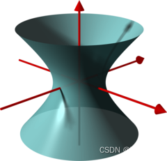
Hyperboloid of one sheet

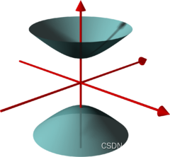
Hyperboloid of two sheets

15 Applications

15.1 Physics

15.1.1 Elliptical reflectors and acoustics

See also: Fresnel zone

If the water’s surface is disturbed at one focus of an elliptical water tank, the circular waves of that disturbance, after reflecting off the walls, converge simultaneously to a single point: the second focus. This is a consequence of the total travel length being the same along any wall-bouncing path between the two foci.

Similarly, if a light source is placed at one focus of an elliptic mirror, all light rays on the plane of the ellipse are reflected to the second focus. Since no other smooth curve has such a property, it can be used as an alternative definition of an ellipse. (In the special case of a circle with a source at its center all light would be reflected back to the center.) If the ellipse is rotated along its major axis to produce an ellipsoidal mirror (specifically, a prolate spheroid), this property holds for all rays out of the source. Alternatively, a cylindrical mirror with elliptical cross-section can be used to focus light from a linear fluorescent lamp along a line of the paper; such mirrors are used in some document scanners.

Sound waves are reflected in a similar way, so in a large elliptical room a person standing at one focus can hear a person standing at the other focus remarkably well. The effect is even more evident under a vaulted roof shaped as a section of a prolate spheroid. Such a room is called a whisper chamber. The same effect can be demonstrated with two reflectors shaped like the end caps of such a spheroid, placed facing each other at the proper distance. Examples are the National Statuary Hall at the United States Capitol (where John Quincy Adams is said to have used this property for eavesdropping on political matters); the Mormon Tabernacle at Temple Square in Salt Lake City, Utah; at an exhibit on sound at the Museum of Science and Industry in Chicago; in front of the University of Illinois at Urbana–Champaign Foellinger Auditorium; and also at a side chamber of the Palace of Charles V, in the Alhambra.

15.1.2 Planetary orbits

Main article: Elliptic orbit
In the 17th century, Johannes Kepler discovered that the orbits along which the planets travel around the Sun are ellipses with the Sun [approximately] at one focus, in his first law of planetary motion. Later, Isaac Newton explained this as a corollary of his law of universal gravitation.

More generally, in the gravitational two-body problem, if the two bodies are bound to each other (that is, the total energy is negative), their orbits are similar ellipses with the common barycenter being one of the foci of each ellipse. The other focus of either ellipse has no known physical significance. The orbit of either body in the reference frame of the other is also an ellipse, with the other body at the same focus.

Keplerian elliptical orbits are the result of any radially directed attraction force whose strength is inversely proportional to the square of the distance. Thus, in principle, the motion of two oppositely charged particles in empty space would also be an ellipse. (However, this conclusion ignores losses due to electromagnetic radiation and quantum effects, which become significant when the particles are moving at high speed.)

For elliptical orbits, useful relations involving the eccentricity {\displaystyle e}e are:

{\displaystyle {\begin{aligned}e&={\frac {r_{a}-r_{p}}{r_{a}+r_{p}}}={\frac {r_{a}-r_{p}}{2a}}\r_{a}&=(1+e)a\r_{p}&=(1-e)a\end{aligned}}}{\displaystyle {\begin{aligned}e&={\frac {r_{a}-r_{p}}{r_{a}+r_{p}}}={\frac {r_{a}-r_{p}}{2a}}\r_{a}&=(1+e)a\r_{p}&=(1-e)a\end{aligned}}}
where

{\displaystyle r_{a}}r_{a} is the radius at apoapsis (the farthest distance)
{\displaystyle r_{p}}r_{p} is the radius at periapsis (the closest distance)
{\displaystyle a}a is the length of the semi-major axis
Also, in terms of {\displaystyle r_{a}}r_{a} and {\displaystyle r_{p}}r_{p}, the semi-major axis {\displaystyle a}a is their arithmetic mean, the semi-minor axis {\displaystyle b}b is their geometric mean, and the semi-latus rectum {\displaystyle \ell }\ell is their harmonic mean. In other words,

{\displaystyle {\begin{aligned}a&={\frac {r_{a}+r_{p}}{2}}\[2pt]b&={\sqrt {r_{a}r_{p}}}\[2pt]\ell &={\frac {2}{{\frac {1}{r_{a}}}+{\frac {1}{r_{p}}}}}={\frac {2r_{a}r_{p}}{r_{a}+r_{p}}}\end{aligned}}}{\displaystyle {\begin{aligned}a&={\frac {r_{a}+r_{p}}{2}}\[2pt]b&={\sqrt {r_{a}r_{p}}}\[2pt]\ell &={\frac {2}{{\frac {1}{r_{a}}}+{\frac {1}{r_{p}}}}}={\frac {2r_{a}r_{p}}{r_{a}+r_{p}}}\end{aligned}}}.

15.1.3 Harmonic oscillators

The general solution for a harmonic oscillator in two or more dimensions is also an ellipse. Such is the case, for instance, of a long pendulum that is free to move in two dimensions; of a mass attached to a fixed point by a perfectly elastic spring; or of any object that moves under influence of an attractive force that is directly proportional to its distance from a fixed attractor. Unlike Keplerian orbits, however, these “harmonic orbits” have the center of attraction at the geometric center of the ellipse, and have fairly simple equations of motion.

15.1.4 Phase visualization

In electronics, the relative phase of two sinusoidal signals can be compared by feeding them to the vertical and horizontal inputs of an oscilloscope. If the Lissajous figure display is an ellipse, rather than a straight line, the two signals are out of phase.

15.1.5 Elliptical gears

Two non-circular gears with the same elliptical outline, each pivoting around one focus and positioned at the proper angle, turn smoothly while maintaining contact at all times. Alternatively, they can be connected by a link chain or timing belt, or in the case of a bicycle the main chainring may be elliptical, or an ovoid similar to an ellipse in form. Such elliptical gears may be used in mechanical equipment to produce variable angular speed or torque from a constant rotation of the driving axle, or in the case of a bicycle to allow a varying crank rotation speed with inversely varying mechanical advantage.

Elliptical bicycle gears make it easier for the chain to slide off the cog when changing gears.[21]

An example gear application would be a device that winds thread onto a conical bobbin on a spinning machine. The bobbin would need to wind faster when the thread is near the apex than when it is near the base.[22]

15.1.6 Optics

In a material that is optically anisotropic (birefringent), the refractive index depends on the direction of the light. The dependency can be described by an index ellipsoid. (If the material is optically isotropic, this ellipsoid is a sphere.)
In lamp-pumped solid-state lasers, elliptical cylinder-shaped reflectors have been used to direct light from the pump lamp (coaxial with one ellipse focal axis) to the active medium rod (coaxial with the second focal axis).[23]
In laser-plasma produced EUV light sources used in microchip lithography, EUV light is generated by plasma positioned in the primary focus of an ellipsoid mirror and is collected in the secondary focus at the input of the lithography machine.[24]

15.2 Statistics and finance

In statistics, a bivariate random vector {\displaystyle (X,Y)}(X,Y) is jointly elliptically distributed if its iso-density contours—loci of equal values of the density function—are ellipses. The concept extends to an arbitrary number of elements of the random vector, in which case in general the iso-density contours are ellipsoids. A special case is the multivariate normal distribution. The elliptical distributions are important in finance because if rates of return on assets are jointly elliptically distributed then all portfolios can be characterized completely by their mean and variance—that is, any two portfolios with identical mean and variance of portfolio return have identical distributions of portfolio return.[25][26]

15.3 Computer graphics

Drawing an ellipse as a graphics primitive is common in standard display libraries, such as the MacIntosh QuickDraw API, and Direct2D on Windows. Jack Bresenham at IBM is most famous for the invention of 2D drawing primitives, including line and circle drawing, using only fast integer operations such as addition and branch on carry bit. M. L. V. Pitteway extended Bresenham’s algorithm for lines to conics in 1967.[27] Another efficient generalization to draw ellipses was invented in 1984 by Jerry Van Aken.[28]

In 1970 Danny Cohen presented at the “Computer Graphics 1970” conference in England a linear algorithm for drawing ellipses and circles. In 1971, L. B. Smith published similar algorithms for all conic sections and proved them to have good properties.[29] These algorithms need only a few multiplications and additions to calculate each vector.

It is beneficial to use a parametric formulation in computer graphics because the density of points is greatest where there is the most curvature. Thus, the change in slope between each successive point is small, reducing the apparent “jaggedness” of the approximation.

Drawing with Bézier paths
Composite Bézier curves may also be used to draw an ellipse to sufficient accuracy, since any ellipse may be construed as an affine transformation of a circle. The spline methods used to draw a circle may be used to draw an ellipse, since the constituent Bézier curves behave appropriately under such transformations.

15.4 Optimization theory

It is sometimes useful to find the minimum bounding ellipse on a set of points. The ellipsoid method is quite useful for solving this problem.

16 See also

Cartesian oval, a generalization of the ellipse
Circumconic and inconic
Distance of closest approach of ellipses
Ellipse fitting
Elliptic coordinates, an orthogonal coordinate system based on families of ellipses and hyperbolae
Elliptic partial differential equation
Elliptical distribution, in statistics
Elliptical dome
Geodesics on an ellipsoid
Great ellipse
Kepler’s laws of planetary motion
n-ellipse, a generalization of the ellipse for n foci
Oval
Spheroid, the ellipsoid obtained by rotating an ellipse about its major or minor axis
Stadium (geometry), a two-dimensional geometric shape constructed of a rectangle with semicircles at a pair of opposite sides
Steiner circumellipse, the unique ellipse circumscribing a triangle and sharing its centroid
Superellipse, a generalization of an ellipse that can look more rectangular or more “pointy”
True, eccentric, and mean anomaly