MATLAB 图像分割

Mayday.603

已于 2022-12-08 10:12:00 修改

阅读量3.7k

点赞数

文章标签： matlab 开发语言图像处理

于 2022-12-08 10:04:17 首次发布

本文链接：https://blog.csdn.net/qq_69604995/article/details/128231584

版权

7.1点检测

代码：

tofloat函数：
```
function [out,revertclass] = tofloat(in)
% tofloat将输入转换为浮点型，使用fft2将会导致标定的问题。
% revertclass将输出类型转化为和输入相同的类型
% 如果输入的图像不是single类型，tofloat将会将其转换为single类型
%
% implement：将所有图像类型以及操作存储起来(cell)，通过函数句柄，将
% 非double和single的函数进行转化，将其转化为single类型的函数(im2single)
%
% revertclass 通过im2xx将其转化为输入的类型
identity = @(x) x;
tosingle = @im2single;

table = {'uint8', tosingle, @im2uint8
'uint16',tosingle,@im2uint16
'int16',tosingle,@im2uint16
'logical',tosingle,@logical
'double',identity,identity
'single',identity,identity};

classIndex = find(strcmp(class(in),table(:,1)));
% class(in) return the type of the input image, then compare with
% the first column in the table(cell).

if isempty(classIndex)
error('Unsupported input image class');
end
% determine whether to find

out = table{classIndex,2}(in);
revertclass=table{classIndex,3};
```
实验代码：

7.2检测指定方向的线

代码：

clc

clear

f=imread('Fig1004(a).tif')

subplot(321);imshow(f)

w=[2 -1 -1;-1 2 -1;-1 -1 2];

g=imfilter(tofloat(f),w);

subplot(322);imshow(g,[])

gtop=g(1:120,1:120);%Top,left section.

gtop=pixeldup(gtop,4);%Enlarge by pixel duplication.

subplot(323);imshow(gtop,[])

gbot =g(end - 119:end, end-119:end);

gbot=pixeldup(gbot,4);

subplot(324);imshow(gbot,[])

g=abs(g);

subplot(325);imshow(g,[])

T=max(g(:));

g=g>=T;

subplot(326);imshow(g)

7.3使用Sobel边缘检测器

代码：

f = imread("Fig1006(a).tif"); % 图像大小：486×486

subplot(3,2,1),imshow(f),title('(a)原始图像');

[gv, t] = edge(f,'sobel','vertical');

subplot(3,2,2),imshow(gv),title('(b)Sobel模板处理后结果');

gv = edge(f, 'sobel', 0.15, 'vertical');

subplot(3,2,3),imshow(gv),title('(c)使用指定阈值的结果');

gboth = edge(f, 'sobel', 0.15);

subplot(3,2,4),imshow(gboth),title('(d)指点阈值确定垂直边缘和水平边缘的结果');

w45 = [-2 -1 0;-1 0 1; 0 1 2];

g45 = imfilter(double(f), w45, 'replicate');

T = 0.3 * max(abs(g45(:)));

g45 = g45 >= T;

subplot(3,2,5),imshow(g45),title('(e)-45°方向边缘');

f45= [0 1 2;-1 0 1;-2 -1 0];

h45= imfilter(double(f), f45,'replicate');

T = 0.3 * max(abs(h45(:)));

h45 = h45 >= T;

subplot(3,2,6),imshow(h45),title('(f)+45°方向边缘');

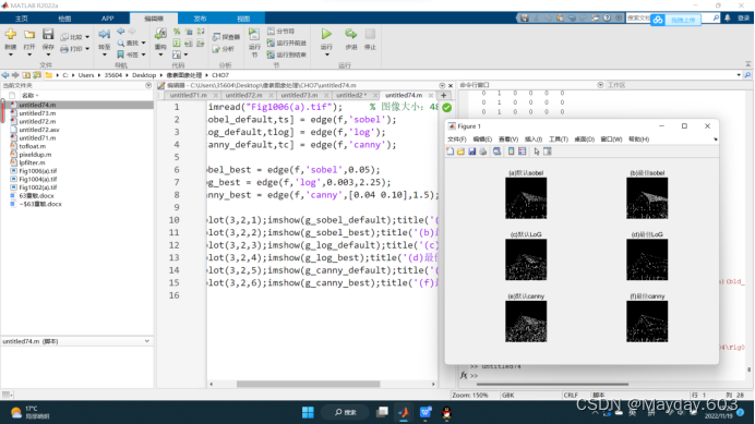
7.4Sobel、LoG和Canny边缘检测器的比较

代码:

f = imread("Fig1006(a).tif"); % 图像大小：486×486

[g_sobel_default,ts] = edge(f,'sobel');

[g_log_default,tlog] = edge(f,'log');

[g_canny_default,tc] = edge(f,'canny');

g_sobel_best = edge(f,'sobel',0.05);

g_log_best = edge(f,'log',0.003,2.25);

g_canny_best = edge(f,'canny',[0.04 0.10],1.5);

subplot(3,2,1);imshow(g_sobel_default);title('(a)默认sobel');

subplot(3,2,2);imshow(g_sobel_best);title('(b)最佳sobel');

subplot(3,2,3);imshow(g_log_default);title('(c)默认LoG');

subplot(3,2,4);imshow(g_log_best);title('(d)最佳LoG');

subplot(3,2,5);imshow(g_canny_default);title('(e)默认canny');

subplot(3,2,6);imshow(g_canny_best);title('(f)最佳canny');

7.5霍夫变换的说明

代码：

f=zeros(101,101);

f(1,1) =1;f(101,1) = 1;f(1,101) = 1;

f(101,101)=1;f(51,51)=1;

subplot(221),imshow(f)

H=hough(f);

subplot(222),imshow(H,[])

[H,theta,rho]=hough(f);

subplot(223),imshow(H,[],'XData',theta,'YData',rho,'InitialMagnification','fit')

axis on,axis normal

xlabel('\theta'),ylabel('\rho')

7.6使用霍夫变换做检测和连接

代码：

f=g_canny_best

[H,theta,rho]=hough(f,'ThetaResolution',0.2);

imshow(H,[],'XData',theta,'YData',rho,'InitialMagnification','fit')

axis on,axis normal

xlabel('\theta'),ylabel('\rho')

peaks=houghpeaks(H,5);

hold on

plot(theta(peaks(:,2)),rho(peaks(:,1)), ...

'LineStyle','none','marker','s','color','w')

lines=houghlines(f,theta,rho,peaks);

figure,imshow(f),hold on

for k=1:length(lines)

xy=[lines(k).point1;lines(k).point2];

plot(xy(:,1),xy(:,2),'LineWidth',4,'Color',[.8 .8 .8]);

end

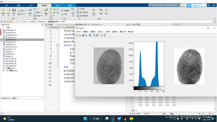
7.7计算全局阈值

代码：

f=imread('Fig1013(a).tif')

count=0;

T=mean2(f);

done=false;

while ~done

count=count+1;

g = f> T;

Tnext=0.5*(mean(f(g))+mean(f(~g)));

done=abs(T-Tnext)<0.5;

T=Tnext;

end

g=im2bw(f,T/255);

subplot(131),imshow(f)

subplot(132),imhist(f)

subplot(133),imshow(g)

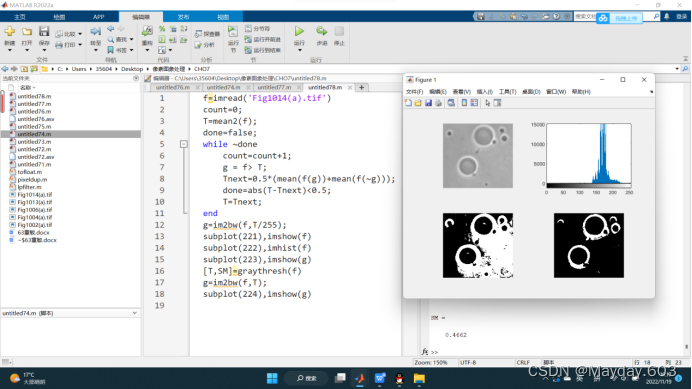
7.8使用Otsu方法和基本全局阈值处理方法分割图像的比较

代码：

f=imread('Fig1014(a).tif')

count=0;

T=mean2(f);

done=false;

while ~done

count=count+1;

g = f> T;

Tnext=0.5*(mean(f(g))+mean(f(~g)));

done=abs(T-Tnext)<0.5;

T=Tnext;

end

g=im2bw(f,T/255);

subplot(221),imshow(f)

subplot(222),imhist(f)

subplot(223),imshow(g)

[T,SM]=graythresh(f)

g=im2bw(f,T);

subplot(224),imshow(g)

7.9使用基于梯度的边缘信息改进全局阈值处理

otsuthresh函数：

function [T,SM]=otsuthresh(h)

h=h/sum(h);

h=h(:);

i=(1:numel(h))';

P1=cumsum(h);

m=cumsum(i.*h);

mG=m(end);

sigSquared=((mG*P1-m).^2)./(P1.*(1-P1)+eps);

maxSigsq=max(sigSquared);

T=mean(find(sigSquared==maxSigsq));

T=(T-1)/(numel(h)-1);

SM=maxSigsq / (sum(((i-mG).^2).*h)+eps);

代码：

f = tofloat(imread("Fig1016(a).tif"));

subplot(231),imshow(f),title('原图像');

subplot(232),imhist(f),title('原图像直方图');

sx = fspecial('sobel');

sy = sx';

gx = imfilter(f,sx,'replicate');

gy = imfilter(f,sy,'replicate');

grad = sqrt(gx.*gx+gy.*gy);

grad = grad/max(grad(:));

h =imhist(grad);

Q = percentile2i(h,0.999);

markerImage = grad>Q;

subplot(233),imshow(markerImage),title('以99.9%进行阈值处理后的梯度幅值图像');

fp = f.*markerImage;

subplot(234),imshow(fp),title('原图像与梯度幅值乘积的图像');

hp = imhist(fp);

hp(1) = 0;

subplot(235),bar(hp),title('原图像与梯度幅值乘积的直方图');

T = otsuthresh(hp);

T*(numel(hp)-1)

g = im2bw(f,T);

subplot(236),imshow(g),title('改进边缘后的图像')
7.10使用拉普拉斯算子边缘信息来改进全局阈值处理

代码：

f = tofloat(imread("Fig1017(a).tif"));

subplot(231),imshow(f),title('原始图像');

subplot(232),imhist(f),title('原始图像的直方图');

hf = imhist(f);

[Tf SMf] = graythresh(f);

gf = im2bw(f,Tf);

subplot(233),imshow(gf),title('对原始图像进行分割的图像');

w= [-1 -1 -1;-1 8 -1;-1 -1 -1];

lap = abs(imfilter(f,w,'replicate'));

lap = lap/max(lap(:));

h = imhist(lap);

Q = percentile2i(h,0.995);

markerImage = lap >Q;

fp = f.*markerImage;

subplot(234),imshow(fp),title('标记图像与原图像的乘积');

hp = imhist(fp);

hp(1) =0;

subplot(235),bar(hp)

T = otsuthresh(hp);

g = im2bw(f,T);a

subplot(236),imshow(g),title('修改边缘后的阈值处理图像')

7.11全局和局部阈值处理的比较

localmean函数：

function mean=localmean(f,nhood)

if nargin==1

nhood=ones(3)/9;

else

nhood=nhood/sum(nhood(:));

end

mean=imfilter(tofloat(f),nhood,'replicate');

end

代码：

f = tofloat(imread("Fig1018(a).tif"));

subplot(2,2,1),imshow(f);title('(a) 酵母细胞的图像');

[TGlobal] = graythresh(f);

gGlobal = im2bw(f, TGlobal);

subplot(2,2,2),imshow(gGlobal);title('(b)用 Otsus 方法分割的图像');

g = localthresh(f, ones(3), 30, 1.5, 'global');

SIG = stdfilt(f, ones(3));

subplot(2,2,3), imshow(SIG, [ ]) ;title('(c) 局部标准差图像');

subplot(2,2,4),imshow(g);title('(d) 用局部阈值处理分割的图像 ');
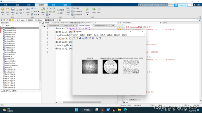
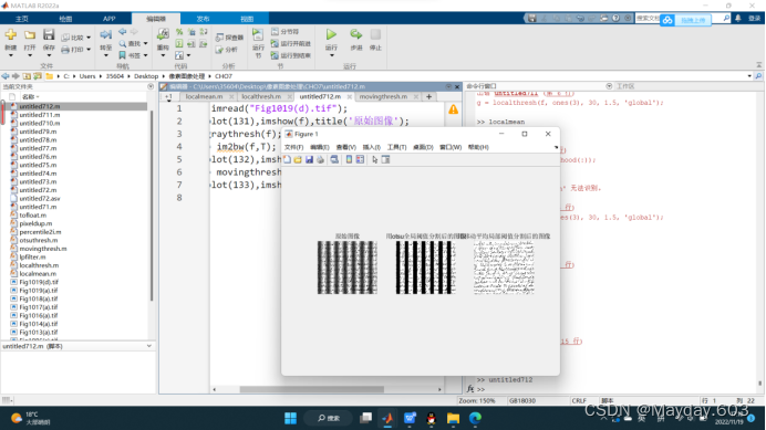
7.12使用移动平均的图像阈值处理

localthresh函数：

function g=localthresh(f,nhood,a,b,meantype)

f=tofloat(f);

SIG=stdfilt(f,nhood);

if nargin==5 && strcmp(meantype,'global')

MEAN=mean2(f);

else

MEAN=localmean(f,nhood);

end

g=(f>a*SIG) & (f>b*MEAN);

end

代码：

f = imread("Fig1019(d).tif");

subplot(131),imshow(f),title('原始图像');

T =graythresh(f);

g1 = im2bw(f,T);

subplot(132),imshow(g1),title('用otsu全局阈值分割后的图像');

g2 = movingthresh(f,20,0.5);

subplot(133),imshow(g2),title('用移动平均局部阈值分割后的图像');

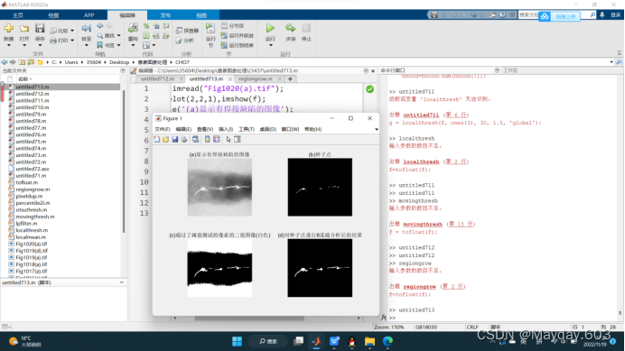
7.13用区域生长检测焊接空隙

regiongrow函数：

function [g,NR,SI,TI]=regiongrow(f,S,T)

f=tofloat(f);

if numel(S)==1

SI=f==S;

S1=S;

else

SI=bwmorph(3,'shrink',Inf);

S1=f(SI);

end

TI=false(size(f));

for K=1:length(S1)

seedvalue=S1(K);

S=abs(f-seedvalue)<=T;

TI=TI|S;

end

[g,NR]=bwlabel(imreconstruct(SI,TI));

代码：

f = imread("Fig1020(a).tif");

subplot(2,2,1),imshow(f);

title('(a)显示有焊接缺陷的图像');

%函数regiongrow返回的NR为是不同区域的数目，参数SI是一副含有种子点的图像

%TI是包含在经过连通前通过阈值测试的像素

[g,NR,SI,TI]=regiongrow(f,1,0.26);%种子的像素值为255，65为阈值

subplot(2,2,2),imshow(SI);

title('(b)种子点');

subplot(2,2,3),imshow(TI);

title('(c)通过了阈值测试的像素的二值图像(白色)');

subplot(2,2,4),imshow(g);

title('(d)对种子点进行8连通分析后的结果');

7.14使用区域分离和聚合的图像分割

splitmerge函数：

function g=splitmerge(f,mindim,fun)%f是待分割的原图，mindim是定义分解中所允许的最小的块，必须是2的正整数次幂

Q=2^nextpow2(max(size(f)));

[M,N]=size(f);

f=padarray(f,[Q-M,Q-N],'post');%：填充图像或填充数组。f是输入图像，输出是填充后的图像，先将图像填充到2的幂次以使后面的分解可行

%然后是填充的行数和列数，post：表示在每一维的最后一个元素后填充,B = padarray(A,padsize,padval,direction)

%不含padval就用0填充,Q代表填充后图像的大小。

S=qtdecomp(f,@split_test,mindim,fun);%S传给split_test，qtdecomp divides a square image into four

% equal-sized square blocks, and then tests each block to see if it

% meets some criterion of homogeneity. If a block meets the criterion,

% it is not divided any further. If it does not meet the criterion,

% it is subdivided again into four blocks, and the test criterion is

% applied to those blocks. This process is repeated iteratively until

% each block meets the criterion. The result can have blocks of several

% different sizes.S是包含四叉树结构的稀疏矩阵，存储的值是块的大小及坐标，以稀疏矩阵形式存储

Lmax=full(max(S(:)));%将以稀疏矩阵存储形式存储的矩阵变换成以普通矩阵（full matrix）形式存储，full，sparse只是存储形式的不同

g=zeros(size(f));

MARKER=zeros(size(f));

for k=1:Lmax

[vals,r,c]=qtgetblk(f,S,k);%vals是一个数组，包含f的四叉树分解中大小为k*k的块的值，是一个k*k*个数的矩阵，

%个数是指S中有多少个这样大小的块，f是被四叉树分的原图像，r，c是对应的左上角块的坐标如2*2块，代表的是左上角开始块的坐标

if ~isempty(vals)

for I=1:length(r)

xlow=r(I);

ylow=c(I);

xhigh=xlow+k-1;

yhigh=ylow+k-1;

region=f(xlow:xhigh,ylow:yhigh);%找到对应的区域

flag=feval(fun,region);%evaluates the function handle, fhandle,using arguments x1 through xn.执行函数fun，region是参数

if flag%如果返回的是1，则进行标记

g(xlow:xhigh,ylow:yhigh)=1;%然后将对应的区域置1

MARKER(xlow,ylow)=1;%MARKER矩阵对应的左上角坐标置1

end

end

end

end

g=bwlabel(imreconstruct(MARKER,g));%imreconstruct默认2D图像8连通，这个函数就是起合的作用

g=g(1:M,1:N);%返回原图像的大小

代码：

f = imread("Fig1023(a).tif");

subplot(231),imshow(f),title('原始图像');

g32 = splitmerge(f,32,@predicate) %使用最小块为32进行分割

subplot(232),imshow(g32),title('使用最小块为32进行分割图像');

g16 = splitmerge(f,16,@predicate) %使用最小块为16进行分割

subplot(233),imshow(g16),title('使用最小块为16进行分割图像');

g8= splitmerge(f,8,@predicate) %使用最小块为8进行分割

subplot(234),imshow(g8),title('使用最小块为8进行分割图像');

g4 = splitmerge(f,4,@predicate) %使用最小块为4进行分割

subplot(235),imshow(g4),title('使用最小块为4进行分割图像');

g2 = splitmerge(f,2,@predicate) %使用最小块为2进行分割

subplot(236),imshow(g2),title('使用最小块为2进行分割图像');

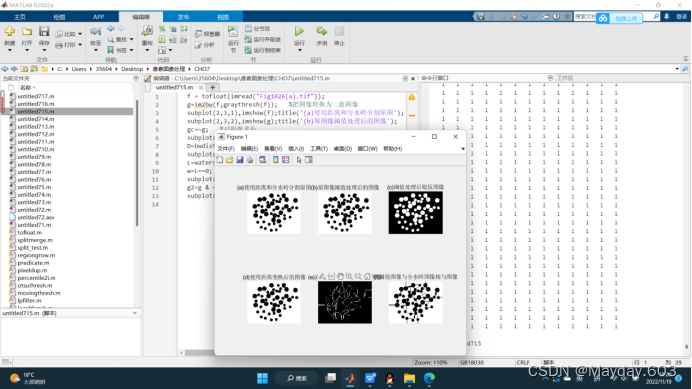
7.15使用距离和分水岭变换分割二值图像

代码:

f = tofloat(imread("Fig1026(a).tif"));

g=im2bw(f,graythresh(f)); %把图像转换为二值图像

subplot(2,3,1),imshow(f);title('(a)使用距离和分水岭分割原图');

subplot(2,3,2),imshow(g);title('(b)原图像阈值处理后的图像');

gc=~g; %对图像求补

subplot(2,3,3),imshow(gc),title('(c)阈值处理后取反图像');

D=bwdist(gc); %计算其距离变换

subplot(2,3,4),imshow(D),title('(d)使用距离变换后的图像');

L=watershed(-D); %计算负距离变换的分水岭变换

w=L==0; %L 的零值即分水岭的脊线像素

subplot(2,3,5),imshow(w),title('(e)距离变换后的负分水岭图像');

g2=g & ~w; %原始二值图像和图像 w 的 “补” 的逻辑 “与” 操作可完成分割

subplot(2,3,6),imshow(g2),title('(f)阈值图像与分水岭图像相与图像');

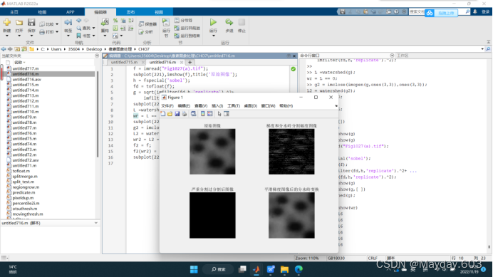
7.16使用梯度和分水岭变换分割灰度图像

代码：

f = imread("Fig1027(a).tif");

subplot(221),imshow(f),title('原始图像');

h = fspecial('sobel');

fd = tofloat(f);

g = sqrt(imfilter(fd,h,'replicate').^2+ ...

imfilter(fd,h,'replicate').^2);

subplot(222),imshow(g,[]),title('梯度和分水岭分割幅度图像');

L =watershed(g);

wr = L == 0;

subplot(223),imshow(wr),title('严重分割过分割后图像');

g2 = imclose(imopen(g,ones(3,3)),ones(3,3));

L2 = watershed(g2);

wr2 = L2 == 0;

f2 = f;

f2(wr2) = 255;

subplot(224),imshow(f2),title('平滑梯度图像后的分水岭变换');

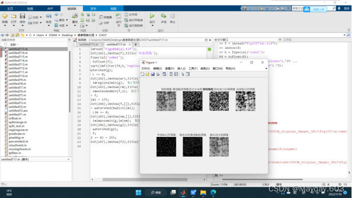
7.17标记符控制的分水岭分割示例

代码：

f = imread("Fig1028(a).tif");

subplot(241),imshow(f),title('原始图像');

h = fspecial('sobel');

fd = tofloat(f);

g = sqrt(imfilter(fd,h,'replicate').^2+imfilter(fd,h,'replicate').^2);

L =watershed(g);

wr = L == 0;

subplot(242),imshow(wr),title('梯度幅度图像进行分水岭变换图像');

rm = imregionalmin(g); %计算图像中所有的局部小区域的位置

subplot(243),imshow(rm),title('梯度幅值的局部小区域图像');

im = imextendedmin(f,2); %用于计算比临近点更暗的图像中“低点”的集合

fim = f;

fim(im) = 175;

subplot(244),imshow(f,[]),title('内部标记符图像');

Lim = watershed(bwdist(im));

em = Lim == 0;

subplot(245),imshow(em,[]),title('外部标记符图像');

g2 = imimposemin(g,im|em); %用来修改一幅图像,使得其只在指定的位置处取得局部最小值

subplot(246),imshow(g2),title('修改后的梯度幅值图像');

L2 = watershed(g2);

f2 = f;

f2(L2 == 0) = 255;

subplot(247),imshow(f2),title('最后的分割图像');

Mayday.603

关注

0
点赞
踩
40

收藏

觉得还不错? 一键收藏
1
评论
MATLAB 图像分割

7.1点检测代码：实验代码：7.2检测指定方向的线代码：clcclearf=imread('Fig1004(a).tif')subplot(321);imshow(f)w=[2 -1 -1;-1 2 -1;-1 -1 2];g=imfilter(tofloat(f),w);subplot(322);imshow(g,[])gtop=g(1:120,1:120);%Top,left section.gtop=pixeldup(gtop,4);%Enlarge by pixel duplication.
复制链接

扫一扫