


一、原理
1.1 引例
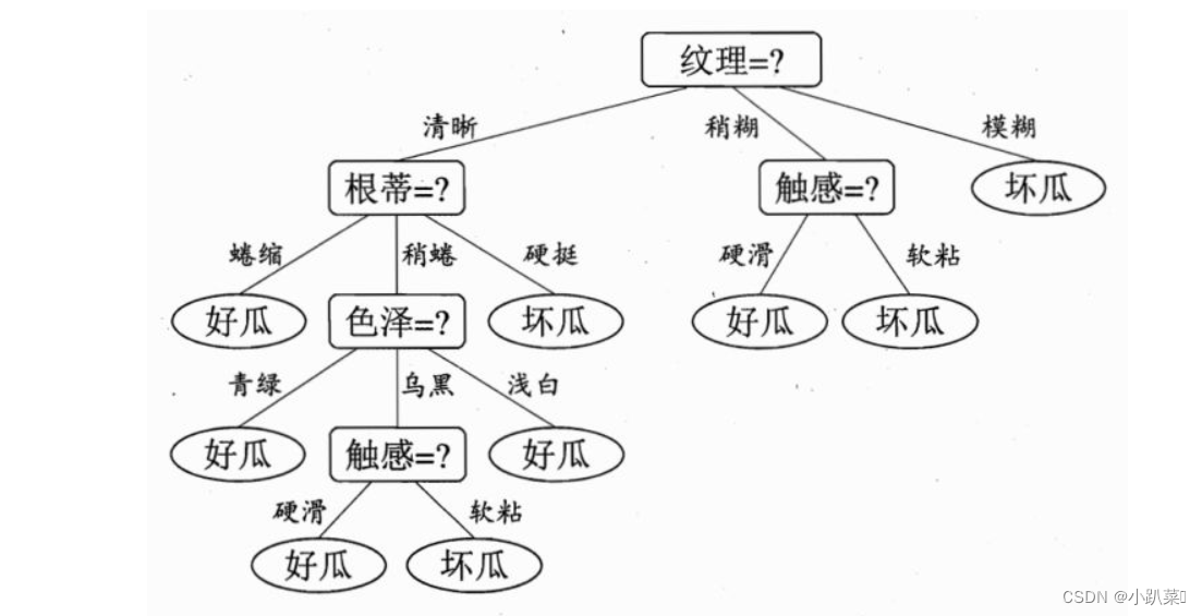
一颗完整的决策树包含以下三个部分:
(1)根节点:就是树最顶端的节点,比如上面图中的“色泽”。
(2)叶子节点:树最底部的那些节点,也就是决策结果,好瓜还是坏瓜。
(3)内部节点,除了叶子结点,都是内部节点。
树中每个内部节点表示在一个属性特征上的测试,每个分支代表一个测试输出,每个叶节点表示一种类别。
给定一个决策树的实例: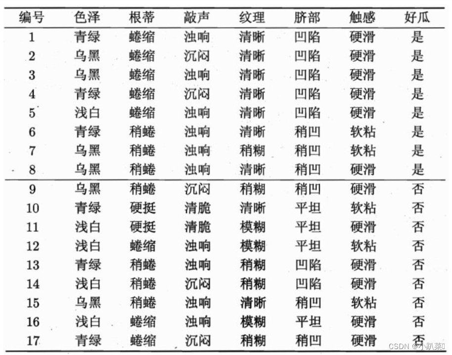
构建的决策树如下:
第一层
根节点:被分成17份,8是/9否,总体的信息熵为:

第二层:
清晰:被分成9份,7是/2否,它的信息熵为:

稍糊:被分成5份,1是/4否,它的信息熵为:

模糊:被分成3份,0是/3否,它的信息熵为:

我们规定,假设我们选取纹理为分类依据,把它作为根节点,那么第二层的加权信息熵可以定义为:
我们规定,H’< H0,也就是随着决策的进行,其不确定度要减小才行,决策肯定是一个由不确定到确定状态的转变。
因此,决策树采用的是自顶向下的递归方法,其基本思想是以信息熵为度量构造一棵熵值下降最快的树,到叶子节点处的熵值为0,此时每个叶子节点中的实例都属于同一类。
1.2 生成算法
构建决策树时首先要确定根节点,而确定方法有以下三种
1.2.1 ID3(信息增益)
从信息论的知识中我们知道:信息熵越大,样本的纯度越低。ID3 算法的核心思想就是以信息增益来度量特征选择,选择信息增益最大的特征进行分裂。
信息增益 = 信息熵 - 条件熵:
也可以表示为H0 - H1,比如上面实例中我选择纹理作为根节点,将根节点一分为三,则:
Gain(D,纹理)=0.998-0.617=0.381)
意思是,没有选择纹理特征前,是否是好瓜的信息熵为0.998,在我选择了纹理这一特征之后,信息熵下降为0.617,信息熵下降了0.381,也就是信息增益为0.381。
由此不断选择信息熵下降最多的作为结点进行划分。
1.2.2 C4.5(信息增益率)
C4.5算法最大的特点是克服了ID3对特征数目的偏重这一缺点,引入信息增益率来作为分类标准。
信息增益率=信息增益/特征本身的熵:

信息增益率对可取值较少的特征有所偏好(分母越小,整体越大),因此C4.5并不是直接用增益率最大的特征进行划分,而是使用一个启发式方法:先从候选划分特征中找到信息增益高于平均值的特征,再从中选择增益率最高的。
例如上述的例子,我们考虑纹理本身的熵,也就是是否是好瓜的熵。
纹理本身有三种可能(9清晰,5稍糊,3模糊),每种概率都已知,则纹理的熵为:

那么选择纹理作为分类依据时,信息增益率为:

1.2.3 基尼指数
基尼指数(基尼不纯度):表示在样本集合中一个随机选中的样本被分错的概率。
基尼系数越小,不纯度越低,特征越好。这和信息增益(率)正好相反。基尼指数可以用来度量任何不均匀分布,是介于0-1之间的数,0是完全相等,1是完全不相等。

1.3算法实例
下面将对三种算法都应用到实力当中
1.3.1ID3算法实例
对一个简单的示例数据集进行分类。在这个示例中,我们使用了一个包含两个特征的数据集,特征的取值范围在0到7之间,目标变量为二元分类,取值为0或1。
import numpy as np

class Node:
    def __init__(self, feature=None, threshold=None, left=None, right=None, value=None):
        self.feature = feature  # 用于分裂的特征索引
        self.threshold = threshold  # 特征的分裂阈值
        self.left = left  # 左子节点
        self.right = right  # 右子节点
        self.value = value  # 叶节点的类别值

class DecisionTree:
    def __init__(self, max_depth=None):
        self.max_depth = max_depth

    def fit(self, X, y):
        self.root = self._build_tree(X, y, depth=0)

    def _build_tree(self, X, y, depth):
        if depth == self.max_depth or len(np.unique(y)) == 1:
            return Node(value=np.bincount(y).argmax())

        n_samples, n_features = X.shape
        best_feature, best_threshold = None, None
        best_info_gain = -np.inf

        for feature in range(n_features):
            thresholds = np.unique(X[:, feature])
            for threshold in thresholds:
                left_indices = np.where(X[:, feature] <= threshold)[0]
                right_indices = np.where(X[:, feature] > threshold)[0]

                if len(left_indices) == 0 or len(right_indices) == 0:
                    continue

                info_gain = self._information_gain(y, y[left_indices], y[right_indices])
                if info_gain > best_info_gain:
                    best_info_gain = info_gain
                    best_feature = feature
                    best_threshold = threshold

        if best_info_gain == 0:
            return Node(value=np.bincount(y).argmax())

        left_indices = np.where(X[:, best_feature] <= best_threshold)[0]
        right_indices = np.where(X[:, best_feature] > best_threshold)[0]

        left_node = self._build_tree(X[left_indices], y[left_indices], depth + 1)
        right_node = self._build_tree(X[right_indices], y[right_indices], depth + 1)

        return Node(feature=best_feature, threshold=best_threshold, left=left_node, right=right_node)

    def _information_gain(self, parent, left_child, right_child):
        p = len(left_child) / len(parent)
        return self._entropy(parent) - p * self._entropy(left_child) - (1 - p) * self._entropy(right_child)

    def _entropy(self, y):
        _, counts = np.unique(y, return_counts=True)
        probabilities = counts / len(y)
        return -np.sum(probabilities * np.log2(probabilities))

    def predict(self, X):
        return np.array([self._traverse_tree(x, self.root) for x in X])

    def _traverse_tree(self, x, node):
        if node.value is not None:
            return node.value

        if x[node.feature] <= node.threshold:
            return self._traverse_tree(x, node.left)
        else:
            return self._traverse_tree(x, node.right)

# 示例数据
X_train = np.array([
    [0, 1],
    [1, 2],
    [2, 3],
    [3, 4],
    [4, 5],
    [5, 6],
    [6, 7],
    [7, 8]
])
y_train = np.array([0, 0, 0, 1, 1, 1, 1, 1])

# 构建并训练决策树模型
tree = DecisionTree(max_depth=3)
tree.fit(X_train, y_train)

# 预测示例
X_test = np.array([[2, 2], [5, 5]])
predictions = tree.predict(X_test)
print(predictions)
1.3.2C4.5算法实例
这个示例中,我们对ID3算法的代码稍作修改,引入了信息增益比的计算,并且将其命名为C4.5算法。C4.5算法与ID3算法的主要区别在于选择最佳特征时使用的评价指标,以及处理缺失值的能力。
import numpy as np

class Node:
    def __init__(self, feature=None, threshold=None, left=None, right=None, value=None):
        self.feature = feature  # 用于分裂的特征索引
        self.threshold = threshold  # 特征的分裂阈值
        self.left = left  # 左子节点
        self.right = right  # 右子节点
        self.value = value  # 叶节点的类别值

class DecisionTree:
    def __init__(self, max_depth=None):
        self.max_depth = max_depth

    def fit(self, X, y):
        self.root = self._build_tree(X, y, depth=0)

    def _build_tree(self, X, y, depth):
        if depth == self.max_depth or len(np.unique(y)) == 1:
            return Node(value=np.bincount(y).argmax())

        n_samples, n_features = X.shape
        best_feature, best_threshold = None, None
        best_info_gain_ratio = -np.inf

        for feature in range(n_features):
            thresholds = np.unique(X[:, feature])
            for threshold in thresholds:
                left_indices = np.where(X[:, feature] <= threshold)[0]
                right_indices = np.where(X[:, feature] > threshold)[0]

                if len(left_indices) == 0 or len(right_indices) == 0:
                    continue

                info_gain = self._information_gain(y, y[left_indices], y[right_indices])
                split_info = self._split_information(y, y[left_indices], y[right_indices])
                info_gain_ratio = info_gain / split_info

                if info_gain_ratio > best_info_gain_ratio:
                    best_info_gain_ratio = info_gain_ratio
                    best_feature = feature
                    best_threshold = threshold

        if best_info_gain_ratio == 0:
            return Node(value=np.bincount(y).argmax())

        left_indices = np.where(X[:, best_feature] <= best_threshold)[0]
        right_indices = np.where(X[:, best_feature] > best_threshold)[0]

        left_node = self._build_tree(X[left_indices], y[left_indices], depth + 1)
        right_node = self._build_tree(X[right_indices], y[right_indices], depth + 1)

        return Node(feature=best_feature, threshold=best_threshold, left=left_node, right=right_node)

    def _information_gain(self, parent, left_child, right_child):
        p = len(left_child) / len(parent)
        return self._entropy(parent) - p * self._entropy(left_child) - (1 - p) * self._entropy(right_child)

    def _entropy(self, y):
        _, counts = np.unique(y, return_counts=True)
        probabilities = counts / len(y)
        return -np.sum(probabilities * np.log2(probabilities))

    def _split_information(self, parent, left_child, right_child):
        p_left = len(left_child) / len(parent)
        p_right = len(right_child) / len(parent)
        return -p_left * np.log2(p_left) - p_right * np.log2(p_right)

    def predict(self, X):
        return np.array([self._traverse_tree(x, self.root) for x in X])

    def _traverse_tree(self, x, node):
        if node.value is not None:
            return node.value

        if x[node.feature] <= node.threshold:
            return self._traverse_tree(x, node.left)
        else:
            return self._traverse_tree(x, node.right)

# 示例数据
X_train = np.array([
    [0, 1],
    [1, 2],
    [2, 3],
    [3, 4],
    [4, 5],
    [5, 6],
    [6, 7],
    [7, 8]
])
y_train = np.array([0, 0, 0, 1, 1, 1, 1, 1])

# 构建并训练决策树模型
tree = DecisionTree(max_depth=3)
tree.fit(X_train, y_train)

# 预测示例
X_test = np.array([[2, 2], [5, 5]])
predictions = tree.predict(X_test)
print(predictions)
二.总结
决策树是一种基本的机器学习算法,其核心思想是通过对数据集进行递归的二分来构建一棵树形结构,每个节点代表一个属性测试,每个分支代表一个测试结果,每个叶子节点代表一个类别或者值。
决策树的关键点包括:
-
可解释性: 决策树的模型结构直观易懂,可以被解释为一系列简单的规则,因此对于决策推理过程的可解释性较强。
-
特征选择: 决策树的关键在于如何选择每个节点的分裂特征,常用的特征选择指标包括信息增益、信息增益比、基尼系数等。
-
剪枝: 决策树容易出现过拟合的问题,为了提高泛化能力,需要对生成的决策树进行剪枝操作,减少决策树的复杂度。
-
连续值和缺失值处理: 决策树算法通常需要对连续值和缺失值进行处理,C4.5算法引入了对连续值的处理和处理缺失值的能力。
-
集成学习: 决策树也常被用于集成学习中的 Bagging、Random Forest 和 Boosting 等算法中,以提高模型的性能。
-
适用性: 决策树适用于分类问题和回归问题,且能够处理多类别分类和多输出回归问题。
-
优缺点: 决策树的优点包括易于理解和解释、对数据的预处理要求低、能够处理数值型和类别型数据等;缺点包括容易过拟合、对噪声敏感、不稳定性等。
综上所述,决策树是一种强大而灵活的机器学习算法,在实际应用中具有广泛的应用场景,并且可以通过各种技术手段进行改进和优化。


 1058
1058


 被折叠的 条评论
为什么被折叠?
被折叠的 条评论
为什么被折叠?
 到【灌水乐园】发言


