随机森林-科比生涯数据集分析与预测

最新推荐文章于 2024-05-23 10:50:55 发布

35仍未老

最新推荐文章于 2024-05-23 10:50:55 发布

阅读量2.6k

点赞数 3

分类专栏：机器学习算法文章标签：机器学习数据挖掘

本文链接：https://blog.csdn.net/quanhujing/article/details/107489413

版权

机器学习算法专栏收录该内容

5 篇文章 23 订阅

订阅专栏

前言

最近想学习一下随机森林，从网上找了一些例子，由于sk-learn版本变更，做了些修改才正常跑起来。本文利用随机森林算法训练出一个预测科比投篮模型。主要用了python的numpy，pandas，matplotlib和sklearn库。

二、设计思路

先来看看这份科比生涯的数据集：

è¿éåå¾çæè¿°

这个表格记录了科比30000多个镜头的详细数据，共有25个标签。

具体的设计思路是将这25个标签代表的数据进行分析，找出对科比投篮结果有影响的标签，利用机器学习中随机森林的算法训练出可以预测科比是否能够投篮命中的模型。

先来看看这25个标签具体代表什么(自己不是篮球的专业人士和爱好者，所以具体的内容可能有所出入，不过不会影响到分析结果)

一、动作类：action_type（用什么方式投的篮）、combined_shot_type（结合什么方式投篮）、game_event_id（游戏事件ID）

二、区域类型：lat（投篮的经度）、loc_x （投篮的x坐标）、loc_y（投篮的y坐标）、lon（投篮的纬度）、shot_zone_area（投篮区域的表示方法一）、shot_zone_basic（投篮区域的表示方法二）、shot_zone_range（投篮区域的表示方法三）、shot_distance（投篮离篮筐的的距离）

三、时间类型：minutes_remaining（离比赛结束还有多少分钟）、 period（第几场）、playoffs（是不是季后赛）、season（赛季）、seconds_remaining（离比赛结束还有多少秒）、game_date（比赛时间）

四、团队类型：game_id（游戏ID）、shot_made_flag （是不是进球了(主要的标签)）、shot_type（2分球还是3分球区域）
team_id（队伍ID）、team_name（队伍名字）、matchup（比赛双方队伍）、opponent（自己所在队伍名字）、shot_id（镜头ID）
可以看到，这25个标签中对于科比能否投篮命中有一些无关紧要的数据，比如team_id，因为这30000多份样本中全是在湖人队打的，shot_id，game_id等等这个数据也无关紧要，具体的分析将会在下面讲解。

三、数据分析

首先利用pandas导入数据，代码如下：

import pandas as pd

# 导入数据
file_path = "Data/data.csv"
raw = pd.read_csv(file_path)
print(raw.shape)
print(raw.head(3)) # head函数默认打印前五行，如果需要打印更多函数，传入参数即可

运行结果如下：

接下来我们再来分析这一份数据表，由于shot_made_flag这个标签竟然有缺失值，这个表示了科比是否进球了，作为最重要的数据，是不能随意进行填充的，我们必须删除掉这些样本进行下一步的工作，代码如下：

import pandas as pd

# 导入数据
file_path = "Data/data.csv"
raw = pd.read_csv(file_path)
print(raw.shape)

raw = raw[pd.notnull(raw['shot_made_flag'])]
print(raw.shape)

运行结果如下：

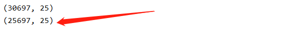
此时我们只有25697个数据进行训练了。

接着我们分析lat，loc_x，loc_y，lon这4个标签，这4个标签说明了科比投篮的位置，而具体指的是什么呢，有什么关系吗，我们画散点图来看一下。

编写代码如下:

import pandas as pd
import matplotlib.pyplot as plt

# 导入数据
file_path = "Data/data.csv"
raw = pd.read_csv(file_path)

# 删除shot_made_flag 为空的数据项，并且命名为kobe训练
kobe = raw[pd.notnull(raw['shot_made_flag'])]

# 画散点图来分析lat loc_x, loc_y, lon这四个标签
alpha = 0.2 # 指定一个数字，用于透明度
plt.figure(figsize=(6,6)) # 指定画图区域
# loc_x 和 loc_y
plt.subplot(121)  # 一行两列，第一个位置
plt.scatter(kobe.loc_x, kobe.loc_y,color='R', alpha=alpha)
plt.title("loc_x and loc_y")
# lat and lon
plt.subplot(122) # 一行两列，第二个位置
plt.scatter(kobe.lon,kobe.lat, color='B', alpha=alpha)
plt.title("lat and lon")
plt.show()

运行结果如图所示:

大致可以看出，这4个坐标大致表示了距离篮筐的距离，那样的话，我们接下来用于数据处理的时候选择其中的一组数据即可了。

shot_type，shot_zone_area，shot_zone_basic，shot_zone_range 这4个标签代表了投篮的区域，其实还是说明一件事，这里就不做赘述了，当然shot_zone_area，shot_zone_basic，shot_zone_range这3个标签将投篮区域相比于shot_type来说分的更细，直接删掉是不是会有问题，其实大可不必担心，因为，接下来我们将会用极坐标的形式表示科比的投篮位置，将更会细化科比的投篮区域。

四、数据处理

首先处理我们上节所说的极坐标的问题，然后我们会发现算出来的dist和shot_distance竟然具有正相关性。

import pandas as pd
import numpy as np
import matplotlib.pyplot as plt

# 导入数据
file_path = "Data/data.csv"
raw = pd.read_csv(file_path)

# 删除shot_made_flag 为空的数据项，并且命名为kobe训练
kobe = raw[pd.notnull(raw['shot_made_flag'])]

# 对于lat、loc_x,loc_y、lon这4个标签，选取loc_x和loc_y这两个标签，并将其转化为极坐标的形式
# dist 表示离篮筐的距离，angle 表示偷懒的角度，这样将会更好的反应科比偷懒的反应结果
raw['dist'] = np.sqrt(raw['loc_x']**2 + raw['loc_y']**2)
loc_x_zero = raw['loc_x'] == 0
angle = np.array([0] * len(raw))
angle = np.arctan(raw['loc_y'][~loc_x_zero] / raw['loc_x'][~loc_x_zero])
angle[loc_x_zero] = np.pi /2
raw['angle'] = angle

# 画图展示dist和shot_distance 的正相关性
plt.figure(figsize=(5,5))
plt.scatter(raw.dist, raw.shot_distance, c='B')
plt.title("dist and shot_distance")
plt.show()

运行结果如下：

这样我们可以保留其中的一个(这里我们保留了dist这个标签)，接着我们将minutes_remaining和seconds_remaining转化成一个标签remaining_time，然后删除不必要的列，非数值型的转换成onehot编码格式

具体编写代码如下，具体说明在代码注释中：

import pandas as pd
import numpy as np
import matplotlib.pyplot as plt

# 导入数据
file_path = "Data/data.csv"
raw = pd.read_csv(file_path)

# 删除shot_made_flag 为空的数据项，并且命名为kobe训练
kobe = raw[pd.notnull(raw['shot_made_flag'])]

# 对于lat、loc_x,loc_y、lon这4个标签，选取loc_x和loc_y这两个标签，并将其转化为极坐标的形式
# dist 表示离篮筐的距离，angle 表示偷懒的角度，这样将会更好的反应科比偷懒的反应结果
raw['dist'] = np.sqrt(raw['loc_x']**2 + raw['loc_y']**2)
loc_x_zero = raw['loc_x'] == 0
angle = np.array([0] * len(raw))
angle = np.arctan(raw['loc_y'][~loc_x_zero] / raw['loc_x'][~loc_x_zero])
angle[loc_x_zero] = np.pi /2
raw['angle'] = angle


# 对于minutes_remaining:离比赛结束还有多少分钟;seconds_remaining:离比赛结束还有多少秒（0-60），
# 这两个属性我们合成距离比赛结束的时间
raw['remaining_time'] = raw['minutes_remaining']*60 + raw['seconds_remaining']

# 机器学习只能识别数值型的数据
# 将赛季中 'Jan-00' 'Feb-01' 'Mar-02'...'1998-99‘转换成 0 ,1,2,....99
raw['season'] = raw['season'].apply(lambda x:int(x.split('-')[1]))

# 删除对于比赛结果没有影响的数据
drops = ['shot_id','team_id','team_name','shot_zone_area','shot_zone_range','shot_zone_basic','matchup',
         'lon','lat','seconds_remaining','minutes_remaining','shot_distance','loc_x','loc_y','game_event_id',
         'game_id','game_date']
for drop in drops:
    raw = raw.drop(drop, 1)
# 将非数值型的数据转换成one-hot编码的格式，加入到数据中并且将原来的数据删除
categorical_vars = ['action_type','combined_shot_type','shot_type','opponent','period','season']
for var in categorical_vars:
    raw = pd.concat([raw, pd.get_dummies(raw[var], prefix=var)],1)
    raw = raw.drop(var, 1)

print(raw.shape)

运行结果：(30697, 129)

为什么会有129行之多，是因为我们用了onehot编码，具体什么是one-hot编码这里就不做赘述了，感兴趣的可以谷歌或者百度一下。

最后我们总结一下，到底这25个标签还剩下什么，首先除去和比赛结果无关的标签，’shot_id’, ‘team_id’, ‘team_name’, ‘shot_zone_area’, ‘shot_zone_range’, ‘shot_zone_basic’,’matchup’, ‘lon’, ‘lat’, ‘seconds_remaining’, ‘minutes_remaining’，’shot_distance’, , ‘game_event_id’, ‘game_id’, ‘game_date’

然后’loc_x’, ‘loc_y’转换成了极坐标的形式，变成了’dist’,’angle’;’seconds_remaining’和’minutes_remaining’合并成了’remaining_time’。

最后将’action_type’, ‘combined_shot_type’, ‘shot_type’, ‘opponent’, ‘period’, ‘season’转换成one-hot编码格式。

至此我们的数据处理工作基本完成了。

五、利用sklearn来进行数据的处理

具体的思路是利用随机森林分类器配合着交叉验证的方法进行数据的分析，先找到最佳的树的个数和树的深度。

编写代码如下：

import pandas as pd
import numpy as np
import time
import matplotlib.pyplot as plt
from sklearn.ensemble import RandomForestClassifier
from sklearn.model_selection import KFold
from sklearn.metrics import log_loss

# 导入数据
file_path = "Data/data.csv"
raw = pd.read_csv(file_path)

# 删除shot_made_flag 为空的数据项，并且命名为kobe训练
kobe = raw[pd.notnull(raw['shot_made_flag'])]

# 对于lat、loc_x,loc_y、lon这4个标签，选取loc_x和loc_y这两个标签，并将其转化为极坐标的形式
# dist 表示离篮筐的距离，angle 表示偷懒的角度，这样将会更好的反应科比偷懒的反应结果
raw['dist'] = np.sqrt(raw['loc_x']**2 + raw['loc_y']**2)
loc_x_zero = raw['loc_x'] == 0
angle = np.array([0] * len(raw))
angle[~loc_x_zero] = np.arctan(raw['loc_y'][~loc_x_zero] / raw['loc_x'][~loc_x_zero])
angle[loc_x_zero] = np.pi /2
raw['angle'] = angle


# 对于minutes_remaining:离比赛结束还有多少分钟;seconds_remaining:离比赛结束还有多少秒（0-60），
# 这两个属性我们合成距离比赛结束的时间
raw['remaining_time'] = raw['minutes_remaining']*60 + raw['seconds_remaining']

# 机器学习只能识别数值型的数据
# 将赛季中 'Jan-00' 'Feb-01' 'Mar-02'...'1998-99‘转换成 0 ,1,2,....99
raw['season'] = raw['season'].apply(lambda x:int(x.split('-')[1]))

# 删除对于比赛结果没有影响的数据
drops = ['shot_id','team_id','team_name','shot_zone_area','shot_zone_range','shot_zone_basic','matchup',
         'lon','lat','seconds_remaining','minutes_remaining','shot_distance','loc_x','loc_y','game_event_id',
         'game_id','game_date']
for drop in drops:
    raw = raw.drop(drop, 1)
# 将非数值型的数据转换成one-hot编码的格式，加入到数据中并且将原来的数据删除
categorical_vars = ['action_type','combined_shot_type','shot_type','opponent','period','season']
for var in categorical_vars:
    raw = pd.concat([raw, pd.get_dummies(raw[var], prefix=var)],1)
    raw = raw.drop(var, 1)

# 将数据分为训练数据和测试数据
train_kobe = raw[pd.notnull(raw['shot_made_flag'])]
train_label = train_kobe['shot_made_flag']
train_kobe = train_kobe.drop('shot_made_flag',1)

test_kobe = raw[pd.isnull(raw['shot_made_flag'])]
test_kobe = test_kobe.drop('shot_made_flag',1)

print('寻找随机森林分类器的最佳树的数量。。。。')
min_score = 100000
best_n = 0
scores_n = []
range_n = np.logspace(0,2, num=10).astype(int)  # 要生成的等步长的样本数量，num默认为50
for n in range_n:
    print("树的数量:{0}".format(n))
    t1 = time.time()
    rfc_score = 0
    rfc = RandomForestClassifier(n_estimators=n)
    for train_k, test_k in KFold(n_splits=10, shuffle=True).split(train_kobe):
        rfc.fit(train_kobe.iloc[train_k], train_label.iloc[train_k])
        pred = rfc.predict(train_kobe.iloc[test_k])
        rfc_score += log_loss(train_label.iloc[test_k], pred)/10
    scores_n.append(rfc_score)
    if rfc_score < min_score:
        min_score = rfc_score
        best_n = n
    t2 = time.time()
    print('建造{0}棵树(耗时1:.3f)秒'.format(n, t2-t1))
print("最佳树的棵树为:{0},得分为:{1}".format(best_n,min_score))

print("寻找随机森林分类器的最佳深度。。。。")
min_score = 100000
best_m = 0
scores_m = []
range_m = np.logspace(0,2,num=10).astype(int)
for m in range_m:
    print("树的最大深度:{0}".format(m))
    t1 = time.time()
    rfc_score = 0
    rfc = RandomForestClassifier(max_depth=m, n_estimators=best_n)
    for train_k, test_k in KFold(n_splits=10, shuffle=True).split(train_kobe):
        rfc.fit(train_kobe.iloc[train_k], train_label.iloc[train_k])
        pred = rfc.predict(train_kobe.iloc[test_k])
        rfc_score += log_loss(train_label.iloc[test_k], pred) /10
    scores_m.append(rfc_score)
    if rfc_score < min_score:
        min_score = rfc_score
        best_m = m
    t2 = time.time()
    print("树的最大深度为:{0}(耗时{1:.3f}秒".format(m, t2-t1))
print("树的最佳深度：{0},得分:{1}".format(best_m, min_score))
# 展示树的棵树变化
plt.figure(figsize=(10,5))
plt.subplot(121)
plt.plot(range_n, scores_n)
plt.ylabel("score")
plt.xlabel("number of trees")
# 展示树的深度变化
plt.subplot(122)
plt.plot(range_m, scores_m)
plt.ylabel('score')
plt.xlabel("max_depth")
plt.show()

运行结果如下，说明当树的颗树为100，并且深度为12的时候，损失函数最小，下面是具体的得分图示。

下面我们用100,12这个参数训练模型，并且预测出5000个’shot_made_flag’的缺失值。

import pandas as pd
import numpy as np
import time
import matplotlib.pyplot as plt
from sklearn.ensemble import RandomForestClassifier
from sklearn.model_selection import KFold
from sklearn.metrics import log_loss

# 导入数据
file_path = "Data/data.csv"
raw = pd.read_csv(file_path)

# 删除shot_made_flag 为空的数据项，并且命名为kobe训练
kobe = raw[pd.notnull(raw['shot_made_flag'])]

# 对于lat、loc_x,loc_y、lon这4个标签，选取loc_x和loc_y这两个标签，并将其转化为极坐标的形式
# dist 表示离篮筐的距离，angle 表示偷懒的角度，这样将会更好的反应科比偷懒的反应结果
raw['dist'] = np.sqrt(raw['loc_x']**2 + raw['loc_y']**2)
loc_x_zero = raw['loc_x'] == 0
angle = np.array([0] * len(raw))
angle[~loc_x_zero] = np.arctan(raw['loc_y'][~loc_x_zero] / raw['loc_x'][~loc_x_zero])
angle[loc_x_zero] = np.pi /2
raw['angle'] = angle


# 对于minutes_remaining:离比赛结束还有多少分钟;seconds_remaining:离比赛结束还有多少秒（0-60），
# 这两个属性我们合成距离比赛结束的时间
raw['remaining_time'] = raw['minutes_remaining']*60 + raw['seconds_remaining']
# 先保存一下shot_id,为接下来的创建result.csv做准备
test_shot_id = raw[pd.isnull(raw['shot_made_flag'])]

# 机器学习只能识别数值型的数据
# 将赛季中 'Jan-00' 'Feb-01' 'Mar-02'...'1998-99‘转换成 0 ,1,2,....99
raw['season'] = raw['season'].apply(lambda x:int(x.split('-')[1]))

# 删除对于比赛结果没有影响的数据
drops = ['shot_id','team_id','team_name','shot_zone_area','shot_zone_range','shot_zone_basic','matchup',
         'lon','lat','seconds_remaining','minutes_remaining','shot_distance','loc_x','loc_y','game_event_id',
         'game_id','game_date']
for drop in drops:
    raw = raw.drop(drop, 1)
# 将非数值型的数据转换成one-hot编码的格式，加入到数据中并且将原来的数据删除
categorical_vars = ['action_type','combined_shot_type','shot_type','opponent','period','season']
for var in categorical_vars:
    raw = pd.concat([raw, pd.get_dummies(raw[var], prefix=var)],1)
    raw = raw.drop(var, 1)

# 将数据分为训练数据和测试数据
train_kobe = raw[pd.notnull(raw['shot_made_flag'])]
train_label = train_kobe['shot_made_flag']
train_kobe = train_kobe.drop('shot_made_flag',1)

test_kobe = raw[pd.isnull(raw['shot_made_flag'])]
test_kobe = test_kobe.drop('shot_made_flag',1)

# 训练模型并且用预测shot_made_flag的缺失值
model = RandomForestClassifier(n_estimators=100, max_depth=12)
model.fit(train_kobe, train_label)
predictions = model.predict(test_kobe)
# result = pd.DataFrame({'shot_id':test_kobe['shot_id'].as_matrix(), 'shot_made_flag':predictions.astype(np.int32)})
result = pd.DataFrame({'shot_id':test_shot_id['shot_id'].as_matrix(),'shot_made_flag':predictions.astype(np.int32)})
result.to_csv("result.csv", index=False)

运行结果如下图:

è¿éåå¾çæè¿°

这里给出了5000个缺失值。

六、总结

本篇文章主要用了机器学习的sklearn库，配合着numpy，pandas，matplotlib的技术路线，利用随机森林算法对科比生涯数据进行分析，对缺失值进行了预测。

参考原文：https://blog.csdn.net/qq_42442369/article/details/86755386

35仍未老

关注

3
点赞
踩
10

收藏

觉得还不错? 一键收藏
打赏
0
评论
随机森林-科比生涯数据集分析与预测

前言最近想学习一下随机森林，从网上找了一些例子，由于sk-learn版本变更，做了些修改才正常跑起来。本文利用随机森林算法训练出一个预测科比投篮模型。主要用了python的numpy，pandas，matplotlib和sklearn库。二、设计思路先来看看这份科比生涯的数据集：这个表格记录了科比30000多个镜头的详细数据，共有25个标签。具体的设计思路是将这25个标签代表的数据进行分析，找出对科比投篮结果有影响的标签，利用机器学习中随机森林的算法训练出可以预测科比是否能够投篮
复制链接

扫一扫