机器学习-特征抽取-核主成分法-Kernel Principal Component(KPCA)

Section I: Brief Introduction on KPCA

Performing a nonlinear mapping via Kernel PCA that transforms the data onto a higher-dimensional space. Then, a standard PCA in this higher-dimensional space to project the data back onto a lower-dimensional space where the samples can be separated by a linear classifier (under the condition that the samples can be separated by density in the input space). However, one downside of this approach is that it is computationally very expensive, and this is where kernel trick is adopted here. The key point lies in that using kernel function, the similarity between two-dimensional feature vectors can be still computed in the original feature space.

FROM
Sebastian Raschka, Vahid Mirjalili. Python机器学习第二版. 南京：东南大学出版社，2018.

Section II: Call KPCA in Sklearn

第一部分：代码

import matplotlib.pyplot as plt
from sklearn import datasets
from sklearn.preprocessing import StandardScaler
from sklearn.model_selection import train_test_split
import numpy as np
from sklearn.linear_model import LogisticRegression
from sklearn.discriminant_analysis import LinearDiscriminantAnalysis as LDA
from PCA.visualize import plot_decision_regions

#Section 1: Prepare data
plt.rcParams['figure.dpi']=200
plt.rcParams['savefig.dpi']=200
font = {'family': 'Times New Roman',
        'weight': 'light'}
plt.rc("font", **font)

#Section 2: Load data and split it into train/test dataset
from sklearn.datasets import make_moons

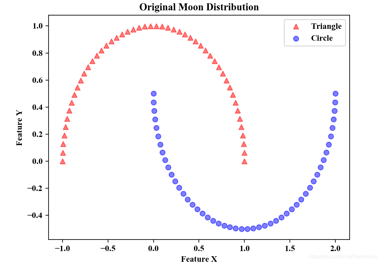
X,y=make_moons(n_samples=100,random_state=12)
plt.scatter(X[y==0,0],X[y==0,1],color='red',marker='^',alpha=0.5,label='Triangle')
plt.scatter(X[y==1,0],X[y==1,1],color='blue',marker='o',alpha=0.5,label='Circle')
plt.legend(loc='best')
plt.xlabel("Feature X")
plt.ylabel('Feature Y')
plt.title("Original Moon Distribution")
plt.savefig('./fig1.png')
plt.show()

#Section 3: Kernal princial component analysis via Sklearn
from sklearn.decomposition import KernelPCA
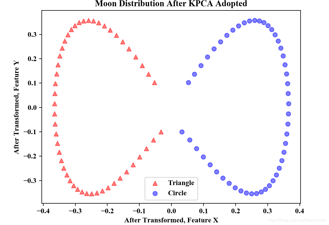
kpca=KernelPCA(n_components=2,kernel='rbf',gamma=15)
X_kpca=kpca.fit_transform(X)
plt.scatter(X_kpca[y==0,0],X_kpca[y==0,1],color='red',marker='^',alpha=0.5,label='Triangle')
plt.scatter(X_kpca[y==1,0],X_kpca[y==1,1],color='blue',marker='o',alpha=0.5,label='Circle')
plt.legend(loc='best')
plt.title("Moon Distribution After KPCA Adopted")
plt.xlabel("After Transformed,Feature X")
plt.ylabel('After Transformed,Feature Y')
plt.savefig('./fig2.png')
plt.show()

第二部分：结果

下图分别为原始Moon的特征分布和采用KPCA后，Moon的特征分布。对比可以得知，采用KPCA将原始空间映射到可划分的高维空间后，进而采取主成分法降维后，所获取的两位特征，显然可以将该问题转变为线性可分的问题。


参考文献：
Sebastian Raschka, Vahid Mirjalili. Python机器学习第二版. 南京：东南大学出版社，2018.