机器学习-非线性关系拟合(Linear, Quadratic和Cubic)

Section I: Code Bundle and Result Analyses

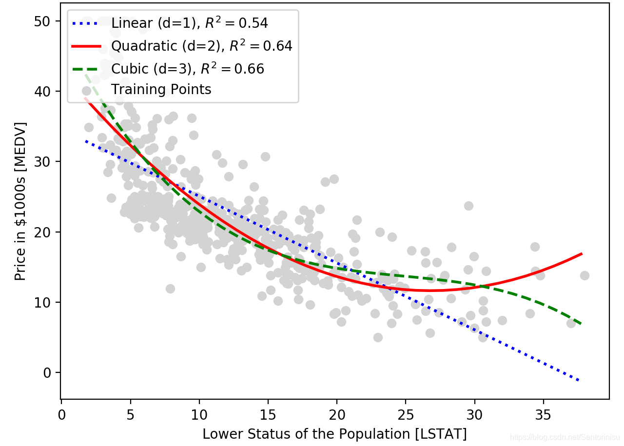
The relationship between house prices and LSTAT(percent lower status of the population) will be fitted via the second degree (quadratic) and the third degree (cubic) polynominals as well as linear fit here.

FROM
Sebastian Raschka, Vahid Mirjalili. Python机器学习第二版. 南京：东南大学出版社，2018.

代码

from sklearn import datasets
from sklearn.model_selection import train_test_split
from sklearn.linear_model import LinearRegression
from sklearn.preprocessing import PolynomialFeatures
from sklearn.metrics import mean_squared_error,r2_score
import matplotlib.pyplot as plt
import numpy as np
import warnings
warnings.filterwarnings("ignore")

plt.rcParams['figure.dpi']=200
plt.rcParams['savefig.dpi']=200
font = {'family': 'Times New Roman',
        'weight': 'light'}
plt.rc("font", **font)

#Section 1: Load data
price=datasets.load_boston()
X=price.data[:,-1]
y=price.target

#Section 2: Create quadratic and cubic polynomial models
quadratic=PolynomialFeatures(degree=2)
cubic=PolynomialFeatures(degree=3)
X_quad=quadratic.fit_transform(X.reshape(-1,1))
X_cubic=cubic.fit_transform(X.reshape(-1,1))

#Section 3: Construct LinearRegression Model and Fit Features
X_fit=np.arange(X.min(),X.max(),1)[:,np.newaxis]

regr=LinearRegression()
regr.fit(X.reshape(-1,1),y)
y_lin_fit=regr.predict(X_fit)
linear_r2=r2_score(y,regr.predict(X.reshape(-1,1)))

regr=regr.fit(X_quad,y)
y_quad_fit=regr.predict(quadratic.fit_transform(X_fit))
quadratic_r2=r2_score(y,regr.predict(X_quad))

regr=regr.fit(X_cubic,y)
y_cubic_fit=regr.predict(cubic.fit_transform(X_fit))
cubic_r2=r2_score(y,regr.predict(X_cubic))

#Section 4: Plot results
plt.scatter(X,y,label='Training Points',color='lightgray')

plt.plot(X_fit,y_lin_fit,
         label='Linear (d=1),$R^2=%.2f$' % linear_r2,
         color='blue',
         lw=2,
         linestyle=':')

plt.plot(X_fit,y_quad_fit,
         label='Quadratic (d=1),$R^2=%.2f$' % quadratic_r2,
         color='red',
         lw=2,
         linestyle='-')

plt.plot(X_fit,y_cubic_fit,
         label='Cubic (d=1),$R^2=%.2f$' % cubic_r2,
         color='green',
         lw=2,
         linestyle='--')

plt.xlabel("Lower Status of the Population [LSTAT]")
plt.ylabel("Price in $1000s [MEDV]")
plt.legend(loc='upper left')
plt.savefig('./fig1.png')
plt.show()

结果

参考文献
Sebastian Raschka, Vahid Mirjalili. Python机器学习第二版. 南京：东南大学出版社，2018.