22&23 - 卷积基础原理与PyTorch卷积API基础功能介绍

22集 - 卷积基础原理与PyTorch卷积API基础功能介绍

22.1 卷积的操作

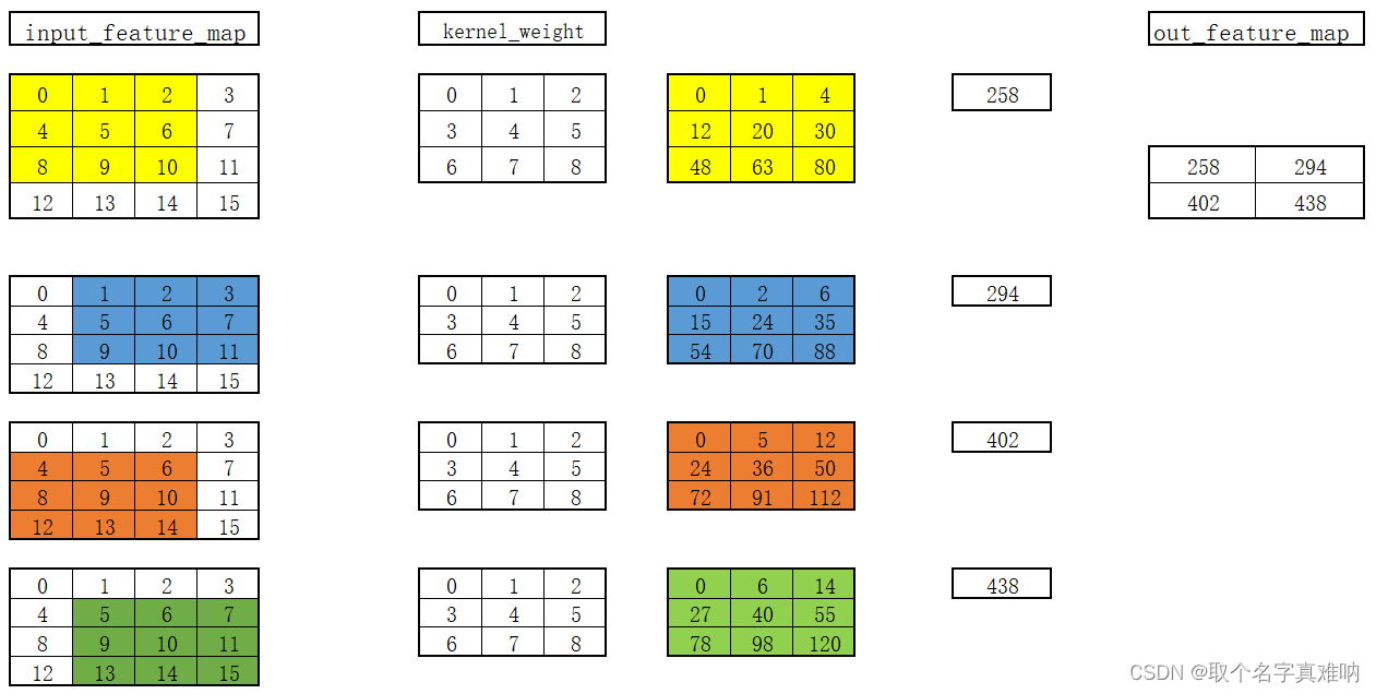
22.2 手动计算

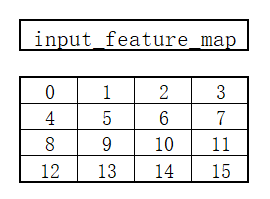
• 定义输入矩阵：
  
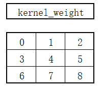
• 定义卷积核权重矩阵
  
• 通过卷积计算可以得到一个输出矩阵
  
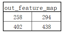
• 具体计算过程如下
  

22.3 代码测试

import torch
from torch import nn
from torch.nn import functional as F

# 定义输入的矩阵
input_feature_map = torch.arange(16,dtype=torch.float).reshape((1,1,4,4))
# 定义输入通道为1
in_channel = 1
# 定义输出通道为1
out_channel =1
# 定义卷积核大小
kernel_size = 3
# 定义卷积核的权重值；kernel_weight.shape = torch.Size([out_channel,in_channel,kernel_height,kernel_width])
kernel_weight = torch.arange(9,dtype=torch.float).reshape(1,1,3,3)
# 通过Conv2d类实例化一个卷积核
my_conv2d = nn.Conv2d(in_channels=in_channel,out_channels=out_channel,kernel_size=kernel_size,bias=False)
# 将卷积核的权重赋值
my_conv2d.weight = nn.Parameter(kernel_weight,requires_grad=True)
# 得到输出特征矩阵，此时用的是nn.Conv2d类处理
output_feature_map = my_conv2d(input_feature_map)
# 得到输出特征矩阵，此时用的是F.conv2d方法处理
functional_output_feature_map = F.conv2d(input_feature_map,kernel_weight)
print(f"input_feature_map={input_feature_map}")
print(f"input_feature_map.shape={input_feature_map.shape}")
print(f"my_conv2d.weight={my_conv2d.weight}")
print(f"my_conv2d.weight.shape={my_conv2d.weight.shape}")
print(f"output_feature_map={output_feature_map}")
print(f"output_feature_map.shape={output_feature_map.shape}")
print(f"functional_output_feature_map={functional_output_feature_map}")
print(f"functional_output_feature_map.shape={functional_output_feature_map.shape}")

input_feature_map=tensor([[[[ 0.,  1.,  2.,  3.],
          [ 4.,  5.,  6.,  7.],
          [ 8.,  9., 10., 11.],
          [12., 13., 14., 15.]]]])
input_feature_map.shape=torch.Size([1, 1, 4, 4])
my_conv2d.weight=Parameter containing:
tensor([[[[0., 1., 2.],
          [3., 4., 5.],
          [6., 7., 8.]]]], requires_grad=True)
my_conv2d.weight.shape=torch.Size([1, 1, 3, 3])
output_feature_map=tensor([[[[258., 294.],
          [402., 438.]]]], grad_fn=<ThnnConv2DBackward>)
output_feature_map.shape=torch.Size([1, 1, 2, 2])
functional_output_feature_map=tensor([[[[258., 294.],
          [402., 438.]]]])
functional_output_feature_map.shape=torch.Size([1, 1, 2, 2])

• 我们通过手动计算的输出矩阵和代码计算得到的矩阵结果一致；

23集 - 基于矩阵滑动相乘逐行实现PyTorch二维卷积

• 基于矩阵滑动相乘逐行计算的二维矩阵对二维矩阵计算

import torch
from torch import nn
from torch.nn import functional as F
import math

# 定义输入的矩阵
input_feature_map = torch.arange(16, dtype=torch.float).reshape((1, 1, 4, 4))
# 定义输入通道为1
in_channel = 1
# 定义输出通道为1
out_channel = 1
# 定义卷积核大小
kernel_size = 3
# 定义卷积核的权重值；kernel_weight.shape = torch.Size([out_channel,in_channel,kernel_height,kernel_width])
kernel_weight = torch.arange(9, dtype=torch.float).reshape(1, 1, 3, 3)
# 通过Conv2d类实例化一个卷积核
my_conv2d = nn.Conv2d(in_channels=in_channel, out_channels=out_channel, kernel_size=kernel_size, bias=False)
# 将卷积核的权重赋值
my_conv2d.weight = nn.Parameter(kernel_weight, requires_grad=True)
# 得到输出特征矩阵，此时用的是nn.Conv2d类处理
output_feature_map = my_conv2d(input_feature_map)
# 得到输出特征矩阵，此时用的是F.conv2d方法处理
functional_output_feature_map = F.conv2d(input_feature_map, kernel_weight)
print(f"input_feature_map={input_feature_map}")
print(f"input_feature_map.shape={input_feature_map.shape}")
print(f"my_conv2d.weight={my_conv2d.weight}")
print(f"my_conv2d.weight.shape={my_conv2d.weight.shape}")
print(f"output_feature_map={output_feature_map}")
print(f"output_feature_map.shape={output_feature_map.shape}")
print(f"functional_output_feature_map={functional_output_feature_map}")
print(f"functional_output_feature_map.shape={functional_output_feature_map.shape}")


# 定义输入矩阵
my_input_matrix = torch.arange(16, dtype=torch.float).reshape(4, 4)
# 定义卷积核矩阵
my_kernel = torch.arange(9, dtype=torch.float).reshape(3, 3)


# 自定义一个矩阵滑动的卷积函数，这里只做二维矩阵和二维矩阵的卷积计算
def matrix_multiplication_for_conv2d(input, kernel, stride=1, padding=0,bias=0):
	# 判断是否需要填充，如果需要，就将上下左右都进行填充指定padding行
	if padding > 0:
		input = F.pad(input, (padding, padding, padding, padding))
	# 得到填充后矩阵的高宽
	input_h, input_w = input.shape
	# 得到卷积核的高宽
	kernel_h, kernel_w = kernel.shape
	# 得到输出矩阵高宽
	output_h = math.floor((input_h - kernel_h) / stride + 1)
	output_w = math.floor((input_w - kernel_w) / stride + 1)
	# 生成一个全0大小的输出矩阵
	output_matrix = torch.zeros(output_h, output_w)
	# 开始遍历，先得到遍历坐标
	for i in range(0, input_h - kernel_h + 1, stride):
		for j in range(0, input_w - kernel_w + 1, stride):
			# 获取遍历的区间region
			region = input[i:i + kernel_h, j: j + kernel_w]
			# 点积后求和得到相应的值
			output_matrix[int(i / stride), int(j / stride)] = torch.sum(region * kernel)+bias

	return output_matrix

# 根据自定义的卷积函数求出输出矩阵
my_output = matrix_multiplication_for_conv2d(my_input_matrix, my_kernel)
# 打印输出结果
print(f"my_output={my_output}")
print(f"判断自定义函数得到的结果是否跟pytorch计算结果一致\n{torch.isclose(my_output,torch.squeeze(functional_output_feature_map))}")
my_input_new = torch.randn(5,5)
my_kernel_weight = torch.randn(3,3)
my_kernel_bias = torch.randn(1)
my_ouput_new = torch.squeeze(F.conv2d(my_input_new.reshape(1,1,5,5),weight=my_kernel_weight.reshape(1,1,3,3),
						bias=my_kernel_bias,stride=2,padding=2))
my_ouput_fun = matrix_multiplication_for_conv2d(my_input_new,my_kernel_weight,stride=2,padding=2,bias=my_kernel_bias)
print(f"my_ouput_new={my_ouput_new}")
print(f"my_ouput_fun={my_ouput_fun}")
print(torch.isclose(my_ouput_new,my_ouput_fun))

• 结果：

input_feature_map=tensor([[[[ 0.,  1.,  2.,  3.],
          [ 4.,  5.,  6.,  7.],
          [ 8.,  9., 10., 11.],
          [12., 13., 14., 15.]]]])
input_feature_map.shape=torch.Size([1, 1, 4, 4])
my_conv2d.weight=Parameter containing:
tensor([[[[0., 1., 2.],
          [3., 4., 5.],
          [6., 7., 8.]]]], requires_grad=True)
my_conv2d.weight.shape=torch.Size([1, 1, 3, 3])
output_feature_map=tensor([[[[258., 294.],
          [402., 438.]]]], grad_fn=<ThnnConv2DBackward>)
output_feature_map.shape=torch.Size([1, 1, 2, 2])
functional_output_feature_map=tensor([[[[258., 294.],
          [402., 438.]]]])
functional_output_feature_map.shape=torch.Size([1, 1, 2, 2])
my_output=tensor([[258., 294.],
        [402., 438.]])
判断自定义函数得到的结果是否跟pytorch计算结果一致
tensor([[True, True],
        [True, True]])
my_ouput_new=tensor([[-1.2405, -0.9159, -1.1279, -1.0144],
        [-3.2825,  0.0432, -0.3291,  0.2662],
        [ 0.0200,  2.7674,  1.8148, -1.2932],
        [-1.3802, -2.4980, -1.6681, -1.0186]])
my_ouput_fun=tensor([[-1.2405, -0.9159, -1.1279, -1.0144],
        [-3.2825,  0.0432, -0.3291,  0.2662],
        [ 0.0200,  2.7674,  1.8148, -1.2932],
        [-1.3802, -2.4980, -1.6681, -1.0186]])
tensor([[True, True, True, True],
        [True, True, True, True],
        [True, True, True, True],
        [True, True, True, True]])