吴恩达machine-learning-specialization2022第2周的optional lab: feature scaling and learing rate

吴天德少侠

已于 2022-10-06 22:28:49 修改

阅读量794

点赞数 1

分类专栏：深度学习 python 文章标签： python 机器学习深度学习

于 2022-10-06 22:26:52 首次发布

本文链接：https://blog.csdn.net/sdhdsf132452/article/details/127188229

版权

python 同时被 2 个专栏收录

89 篇文章 3 订阅

订阅专栏

深度学习

67 篇文章 4 订阅

订阅专栏

1. 目标

调整学习率
使用z-score的数据尺度归一化
z-score: $x=\frac{x-\mu}{\sigma}$

2. dataset

size(sqft)	number of bedrooms	number of floors	age of home	price
952	2	1	65	271.5
1244	3	2	64	232
1947	3	2	17	509.8
…	…	…	…	…

梯度下降

$\begin{align*}\text{repeat}&\text{until convergence:} \;\lbrace \newline\;& w_j :=w_j - \alpha \frac{\partial J(\mathbf{w},b)}{\partial w_j} \tag{1}\; & \text{for j=0..n-1}\newline &b\ \ :=b-\alpha \frac{\partial J(\mathbf{w},b)}{\partial b} \newline \rbrace \end{align*}$

4. 代码

import numpy as np
import matplotlib.pyplot as plt
from lab_utils_multi import (load_house_data,
                    run_gradient_descent,norm_plot,
                    plt_equal_scale,plot_cost_i_w)
from lab_utils_common import dlc            

np.set_printoptions(precision=2)
plt.style.use('deeplearning.mplstyle')

def zscore_norm_features(x):
    """功能: 按列对x进行x-score归一化\n
    返回:\n
    x_norm: 按列归一化后的x\n
    mu: shape=(n,), 每种特征的均值\n
    sigma: shape=(n,), 每种特征的标准差\n
    """
    mu = np.mean(x,axis=0)
    sigma = np.std(x,axis=0)
    x_norm = (x-mu)/sigma

    return x_norm,mu,sigma





if __name__ == '__main__':
    x_train,y_train = load_house_data()
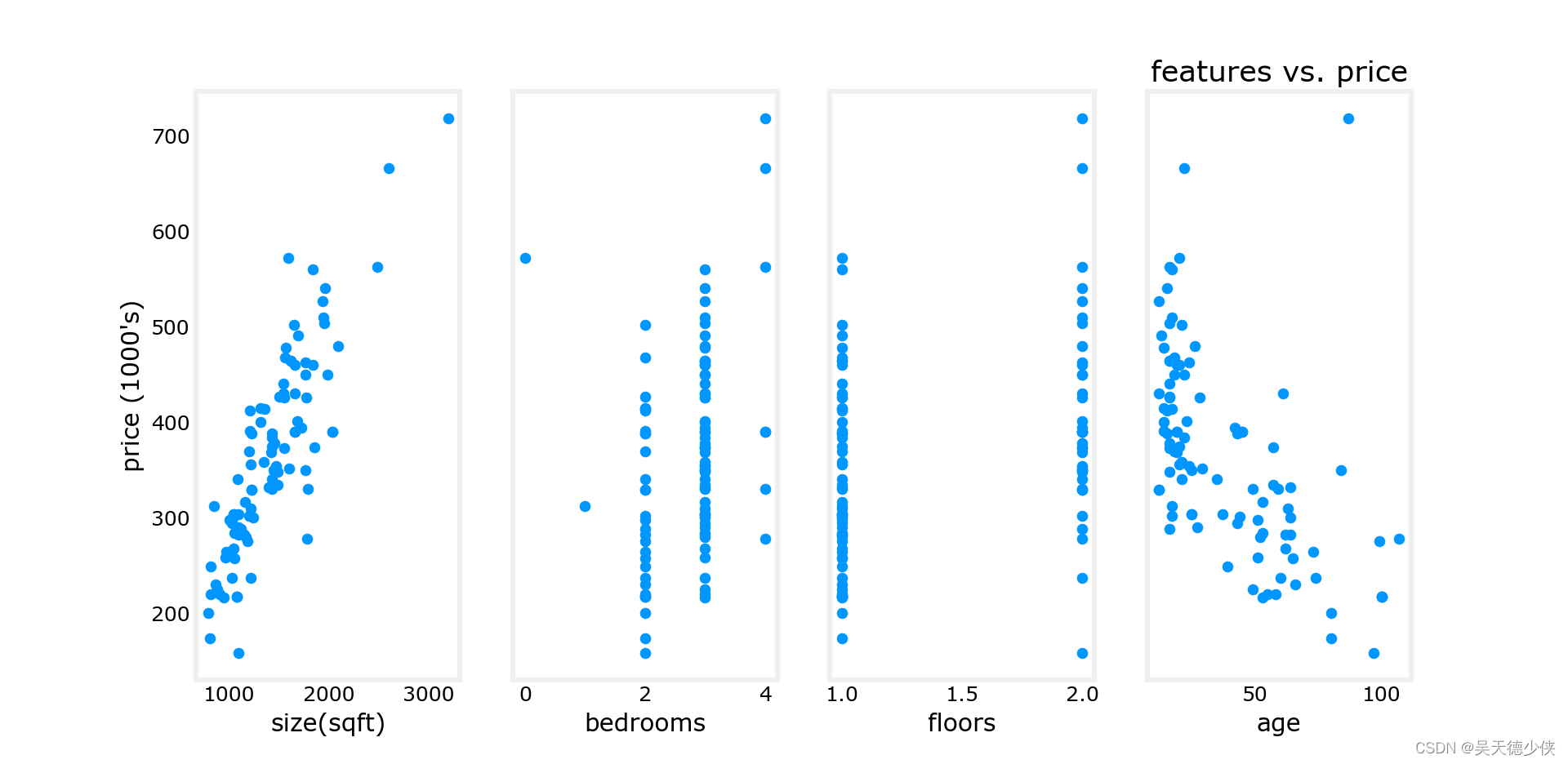
    x_features = ["size(sqft)","bedrooms","floors","age"]

    # 显示每种特征对房价的影响
    # fig,ax = plt.subplots(1,4,figsize=(12,3),sharey=True)
    # for i in range(len(ax)):
    #     ax[i].scatter(x_train[:,i],y_train)
    #     ax[i].set_xlabel(x_features[i])
    # ax[0].set_ylabel("price (1000's)")
    # plt.title('features vs. price')
    # plt.show()

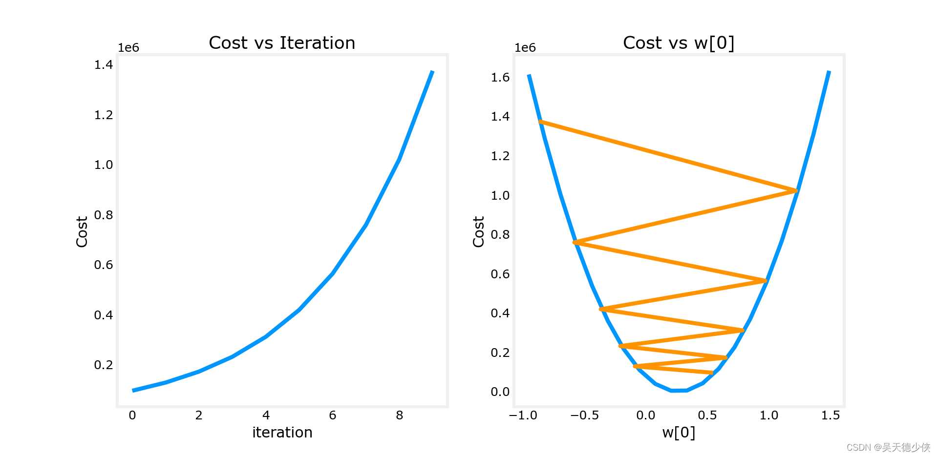
    # 设置alpha为9.9e-7
    # _,_,hist = run_gradient_descent(x_train,y_train,10,alpha=9.9e-7)
    # plot_cost_i_w(x_train,y_train,hist)

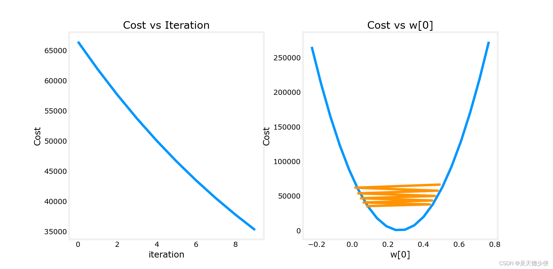
    # alpha设置的小一点: 9e-7
    # _,_,hist = run_gradient_descent(x_train,y_train,10,alpha=9e-7)
    # plot_cost_i_w(x_train,y_train,hist)

    # alpha设置的再小一点: 1e-7
    # _,_,hist = run_gradient_descent(x_train,y_train,10,alpha=1e-7)
    # plot_cost_i_w(x_train,y_train,hist)

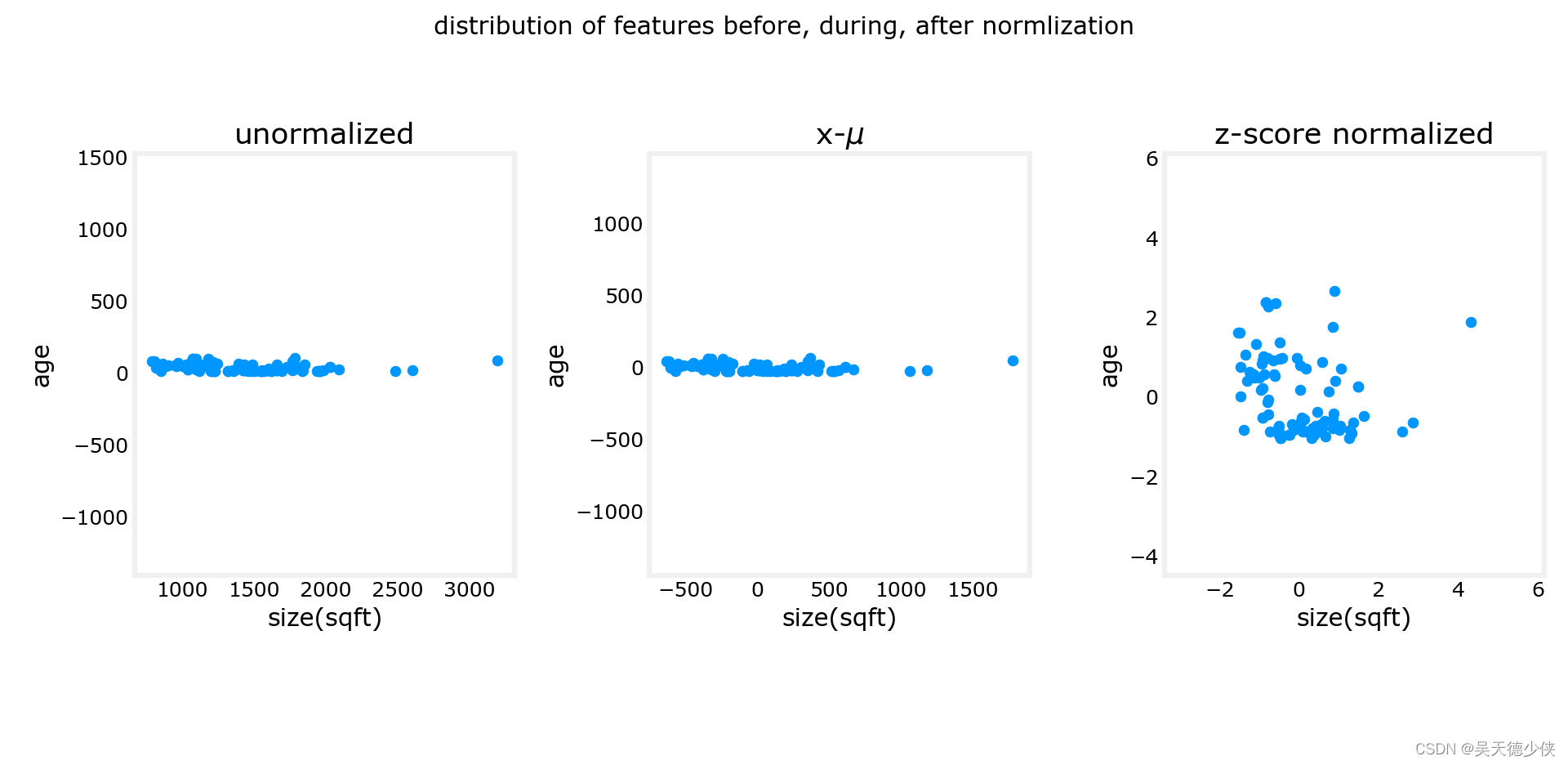
    # 查看归一化后的数据分布
    x_norm,mu,sigma = zscore_norm_features(x_train)
    # fig,ax = plt.subplots(1,3,figsize=(12,3))
    # ax[0].scatter(x_train[:,0],x_train[:,3])
    # ax[0].set_xlabel(x_features[0])
    # ax[0].set_ylabel(x_features[3])
    # ax[0].set_title("unormalized")
    # ax[0].axis('equal')

    # x_mean = x_train-mu
    # ax[1].scatter(x_mean[:,0],x_mean[:,3])
    # ax[1].set_xlabel(x_features[0])
    # ax[1].set_ylabel(x_features[3])
    # ax[1].set_title(r'x-$\mu$')
    # ax[1].axis("equal")

    # ax[2].scatter(x_norm[:,0],x_norm[:,3])
    # ax[2].set_xlabel(x_features[0])
    # ax[2].set_ylabel(x_features[3])
    # ax[2].set_title("z-score normalized")
    # ax[2].axis('equal')

    # plt.tight_layout(rect=[0,0.03,1,0.95])
    # fig.suptitle("distribution of features before, during, after normlization")
    # plt.show()

    # print(f'peak to peak range by column in raw x: {np.ptp(x_train,axis=0)}')
    # print(f'peak to peak range by column in normalized x: {np.ptp(x_norm,axis=0)}')

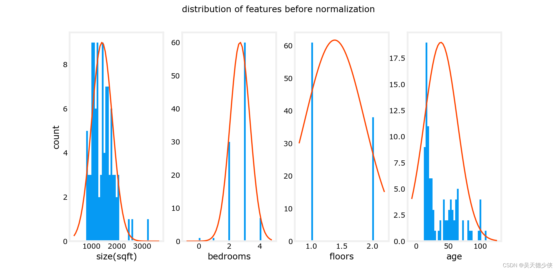
    # 查看peak to peak分布情况
    # fig,ax = plt.subplots(1,4,figsize=(12,3))
    # for i in range(len(ax)):
    #     norm_plot(ax[i],x_train[:,i])
    #     ax[i].set_xlabel(x_features[i])

    # ax[0].set_ylabel("count")
    # fig.suptitle("distribution of features before normalization")
    # # plt.show()

    # fig,ax = plt.subplots(1,4,figsize=(12,3))
    # for i in range(len(ax)):
    #     norm_plot(ax[i],x_norm[:,i])
    #     ax[i].set_xlabel(x_features[i])

    # ax[0].set_ylabel("count")
    # fig.suptitle("distribution of features after normalization")
    # plt.show()

    # 现在使用归一化后的数据，更大的学习率重新做梯度下降优化
    w_norm,b_norm,hist = run_gradient_descent(x_norm,y_train,1000,1.0e-1)
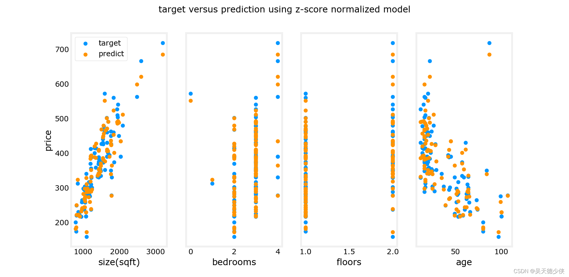
    # 查看预测结果与标签结果
    # m = x_norm.shape[0]
    # yp = np.zeros(m)
    # for i in range(m):
    #     yp[i] = np.dot(x_norm[i],w_norm) + b_norm
    # fig,ax = plt.subplots(1,4,figsize=(12,3),sharey=True)
    # for i in range(len(ax)):
    #     ax[i].scatter(x_train[:,i],y_train,label='target')
    #     ax[i].set_xlabel(x_features[i])
    #     ax[i].scatter(x_train[:,i],yp,color=dlc['dlorange'],label='predict')
    # ax[0].set_ylabel("price")
    # ax[0].legend()
    # fig.suptitle("target versus prediction using z-score normalized model")
    # plt.show()

    # prediction
    # x_house = np.array([1200,3,1,40])
    # x_house_norm = (x_house - mu) - sigma
    # print(x_house_norm)
    # x_house_predict = np.dot(x_house,w_norm) + b_norm
    # print(f'predicted price of a house with 1200 sqrt, \
    #     3 bedrooms, 1 floor 40 years old = ${x_house_predict*1000:.0f}')

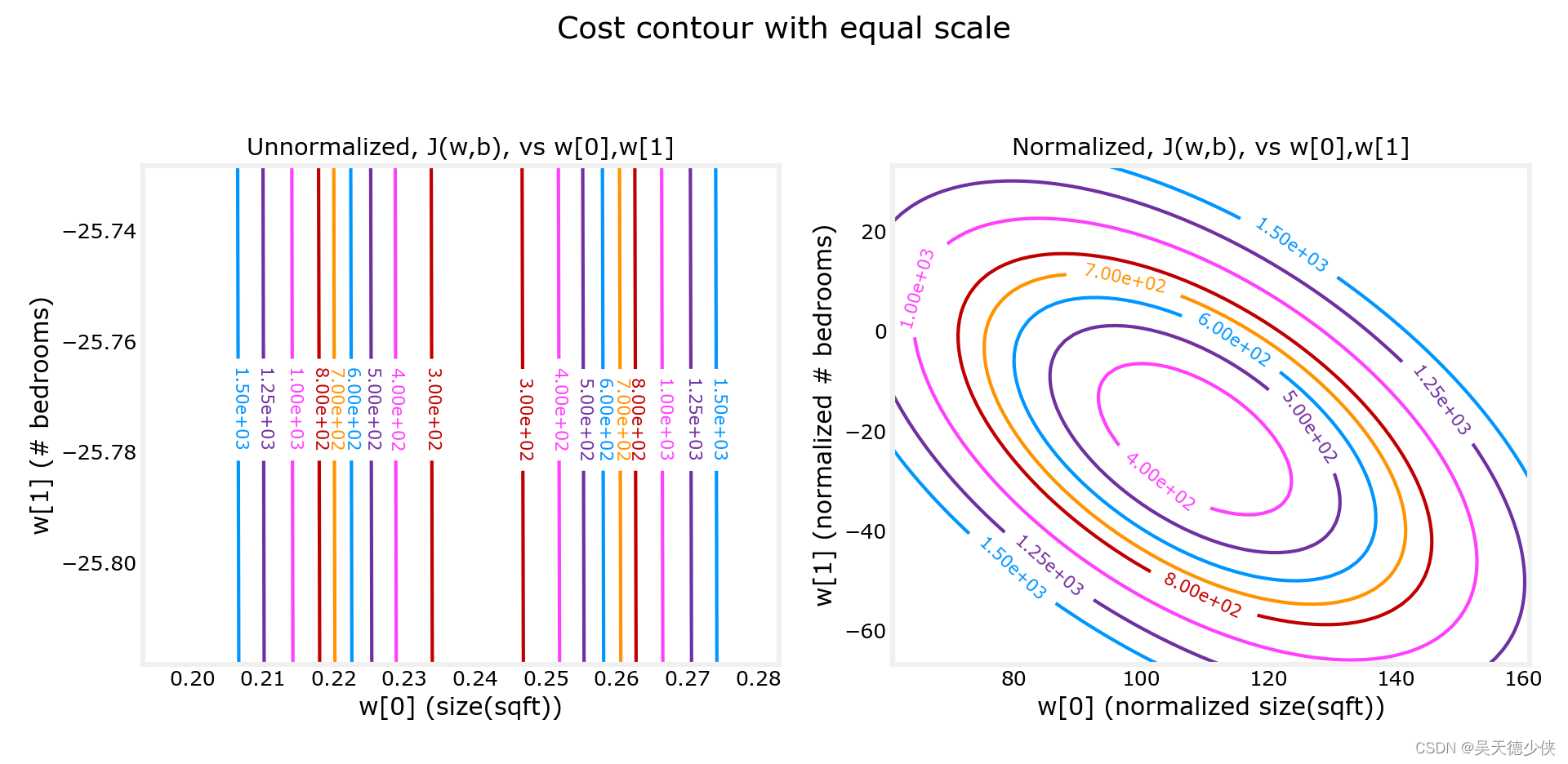
    plt_equal_scale(x_train,x_norm,y_train)

5. 结果

在这里插入图片描述

Iteration Cost          w0       w1       w2       w3       b       djdw0    djdw1    djdw2    djdw3    djdb
---------------------|--------|--------|--------|--------|--------|--------|--------|--------|--------|--------|
0 9.55884e+04  5.5e-01  1.0e-03  5.1e-04  1.2e-02  3.6e-04 -5.5e+05 -1.0e+03 -5.2e+02 -1.2e+04 -3.6e+02
1 1.28213e+05 -8.8e-02 -1.7e-04 -1.0e-04 -3.4e-03 -4.8e-05  6.4e+05  1.2e+03  6.2e+02  1.6e+04  4.1e+02
2 1.72159e+05  6.5e-01  1.2e-03  5.9e-04  1.3e-02  4.3e-04 -7.4e+05 -1.4e+03 -7.0e+02 -1.7e+04 -4.9e+02
3 2.31358e+05 -2.1e-01 -4.0e-04 -2.3e-04 -7.5e-03 -1.2e-04  8.6e+05  1.6e+03  8.3e+02  2.1e+04  5.6e+02
4 3.11100e+05  7.9e-01  1.4e-03  7.1e-04  1.5e-02  5.3e-04 -1.0e+06 -1.8e+03 -9.5e+02 -2.3e+04 -6.6e+02
5 4.18517e+05 -3.7e-01 -7.1e-04 -4.0e-04 -1.3e-02 -2.1e-04  1.2e+06  2.1e+03  1.1e+03  2.8e+04  7.5e+02
6 5.63212e+05  9.7e-01  1.7e-03  8.7e-04  1.8e-02  6.6e-04 -1.3e+06 -2.5e+03 -1.3e+03 -3.1e+04 -8.8e+02
7 7.58122e+05 -5.8e-01 -1.1e-03 -6.2e-04 -1.9e-02 -3.4e-04  1.6e+06  2.9e+03  1.5e+03  3.8e+04  1.0e+03
8 1.02068e+06  1.2e+00  2.2e-03  1.1e-03  2.3e-02  8.3e-04 -1.8e+06 -3.3e+03 -1.7e+03 -4.2e+04 -1.2e+03
9 1.37435e+06 -8.7e-01 -1.7e-03 -9.1e-04 -2.7e-02 -5.2e-04  2.1e+06  3.9e+03  2.0e+03  5.1e+04  1.4e+03

w,b found by gradient descent: w: [-0.87 -0.   -0.   -0.03], b: -0.00

在这里插入图片描述

Iteration Cost          w0       w1       w2       w3       b       djdw0    djdw1    djdw2    djdw3    djdb
---------------------|--------|--------|--------|--------|--------|--------|--------|--------|--------|--------|
        0 6.64616e+04  5.0e-01  9.1e-04  4.7e-04  1.1e-02  3.3e-04 -5.5e+05 -1.0e+03 -5.2e+02 -1.2e+04 -3.6e+02
        1 6.18990e+04  1.8e-02  2.1e-05  2.0e-06 -7.9e-04  1.9e-05  5.3e+05  9.8e+02  5.2e+02  1.3e+04  3.4e+02
        2 5.76572e+04  4.8e-01  8.6e-04  4.4e-04  9.5e-03  3.2e-04 -5.1e+05 -9.3e+02 -4.8e+02 -1.1e+04 -3.4e+02
        3 5.37137e+04  3.4e-02  3.9e-05  2.8e-06 -1.6e-03  3.8e-05  4.9e+05  9.1e+02  4.8e+02  1.2e+04  3.2e+02
        4 5.00474e+04  4.6e-01  8.2e-04  4.1e-04  8.0e-03  3.2e-04 -4.8e+05 -8.7e+02 -4.5e+02 -1.1e+04 -3.1e+02
        5 4.66388e+04  5.0e-02  5.6e-05  2.5e-06 -2.4e-03  5.6e-05  4.6e+05  8.5e+02  4.5e+02  1.2e+04  2.9e+02
        6 4.34700e+04  4.5e-01  7.8e-04  3.8e-04  6.4e-03  3.2e-04 -4.4e+05 -8.1e+02 -4.2e+02 -9.8e+03 -2.9e+02
        7 4.05239e+04  6.4e-02  7.0e-05  1.2e-06 -3.3e-03  7.3e-05  4.3e+05  7.9e+02  4.2e+02  1.1e+04  2.7e+02
        8 3.77849e+04  4.4e-01  7.5e-04  3.5e-04  4.9e-03  3.2e-04 -4.1e+05 -7.5e+02 -3.9e+02 -9.1e+03 -2.7e+02
        9 3.52385e+04  7.7e-02  8.3e-05 -1.1e-06 -4.2e-03  8.9e-05  4.0e+05  7.4e+02  3.9e+02  1.0e+04  2.5e+02
w,b found by gradient descent: w: [ 7.74e-02  8.27e-05 -1.06e-06 -4.20e-03], b: 0.00

在这里插入图片描述

Iteration Cost          w0       w1       w2       w3       b       djdw0    djdw1    djdw2    djdw3    djdb
---------------------|--------|--------|--------|--------|--------|--------|--------|--------|--------|--------|
        0 4.42313e+04  5.5e-02  1.0e-04  5.2e-05  1.2e-03  3.6e-05 -5.5e+05 -1.0e+03 -5.2e+02 -1.2e+04 -3.6e+02
        1 2.76461e+04  9.8e-02  1.8e-04  9.2e-05  2.2e-03  6.5e-05 -4.3e+05 -7.9e+02 -4.0e+02 -9.5e+03 -2.8e+02
        2 1.75102e+04  1.3e-01  2.4e-04  1.2e-04  2.9e-03  8.7e-05 -3.4e+05 -6.1e+02 -3.1e+02 -7.3e+03 -2.2e+02
        3 1.13157e+04  1.6e-01  2.9e-04  1.5e-04  3.5e-03  1.0e-04 -2.6e+05 -4.8e+02 -2.4e+02 -5.6e+03 -1.8e+02
        4 7.53002e+03  1.8e-01  3.3e-04  1.7e-04  3.9e-03  1.2e-04 -2.1e+05 -3.7e+02 -1.9e+02 -4.2e+03 -1.4e+02
        5 5.21639e+03  2.0e-01  3.5e-04  1.8e-04  4.2e-03  1.3e-04 -1.6e+05 -2.9e+02 -1.5e+02 -3.1e+03 -1.1e+02
        6 3.80242e+03  2.1e-01  3.8e-04  1.9e-04  4.5e-03  1.4e-04 -1.3e+05 -2.2e+02 -1.1e+02 -2.3e+03 -8.6e+01
        7 2.93826e+03  2.2e-01  3.9e-04  2.0e-04  4.6e-03  1.4e-04 -9.8e+04 -1.7e+02 -8.6e+01 -1.7e+03 -6.8e+01
        8 2.41013e+03  2.3e-01  4.1e-04  2.1e-04  4.7e-03  1.5e-04 -7.7e+04 -1.3e+02 -6.5e+01 -1.2e+03 -5.4e+01
        9 2.08734e+03  2.3e-01  4.2e-04  2.1e-04  4.8e-03  1.5e-04 -6.0e+04 -1.0e+02 -4.9e+01 -7.5e+02 -4.3e+01
w,b found by gradient descent: w: [2.31e-01 4.18e-04 2.12e-04 4.81e-03], b: 0.00

在这里插入图片描述

peak to peak range by column in raw x: [2.41e+03 4.00e+00 1.00e+00 9.50e+01]
peak to peak range by column in normalized x: [5.85 6.14 2.06 3.69]

在这里插入图片描述

Iteration Cost          w0       w1       w2       w3       b       djdw0    djdw1    djdw2    djdw3    djdb
---------------------|--------|--------|--------|--------|--------|--------|--------|--------|--------|--------|
        0 5.76170e+04  8.9e+00  3.0e+00  3.3e+00 -6.0e+00  3.6e+01 -8.9e+01 -3.0e+01 -3.3e+01  6.0e+01 -3.6e+02
      100 2.21086e+02  1.1e+02 -2.0e+01 -3.1e+01 -3.8e+01  3.6e+02 -9.2e-01  4.5e-01  5.3e-01 -1.7e-01 -9.6e-03
      200 2.19209e+02  1.1e+02 -2.1e+01 -3.3e+01 -3.8e+01  3.6e+02 -3.0e-02  1.5e-02  1.7e-02 -6.0e-03 -2.6e-07
      300 2.19207e+02  1.1e+02 -2.1e+01 -3.3e+01 -3.8e+01  3.6e+02 -1.0e-03  5.1e-04  5.7e-04 -2.0e-04 -6.9e-12
      400 2.19207e+02  1.1e+02 -2.1e+01 -3.3e+01 -3.8e+01  3.6e+02 -3.4e-05  1.7e-05  1.9e-05 -6.6e-06 -2.7e-13
      500 2.19207e+02  1.1e+02 -2.1e+01 -3.3e+01 -3.8e+01  3.6e+02 -1.1e-06  5.6e-07  6.2e-07 -2.2e-07 -2.6e-13
      600 2.19207e+02  1.1e+02 -2.1e+01 -3.3e+01 -3.8e+01  3.6e+02 -3.7e-08  1.9e-08  2.1e-08 -7.3e-09 -2.6e-13
      700 2.19207e+02  1.1e+02 -2.1e+01 -3.3e+01 -3.8e+01  3.6e+02 -1.2e-09  6.2e-10  6.9e-10 -2.4e-10 -2.6e-13
      800 2.19207e+02  1.1e+02 -2.1e+01 -3.3e+01 -3.8e+01  3.6e+02 -4.1e-11  2.1e-11  2.3e-11 -8.1e-12 -2.7e-13
      900 2.19207e+02  1.1e+02 -2.1e+01 -3.3e+01 -3.8e+01  3.6e+02 -1.4e-12  7.0e-13  7.6e-13 -2.7e-13 -2.6e-13
w,b found by gradient descent: w: [110.56 -21.27 -32.71 -37.97], b: 363.16

在这里插入图片描述

Iteration Cost          w0       w1       w2       w3       b       djdw0    djdw1    djdw2    djdw3    djdb
---------------------|--------|--------|--------|--------|--------|--------|--------|--------|--------|--------|
        0 5.76170e+04  8.9e+00  3.0e+00  3.3e+00 -6.0e+00  3.6e+01 -8.9e+01 -3.0e+01 -3.3e+01  6.0e+01 -3.6e+02
      100 2.21086e+02  1.1e+02 -2.0e+01 -3.1e+01 -3.8e+01  3.6e+02 -9.2e-01  4.5e-01  5.3e-01 -1.7e-01 -9.6e-03
      200 2.19209e+02  1.1e+02 -2.1e+01 -3.3e+01 -3.8e+01  3.6e+02 -3.0e-02  1.5e-02  1.7e-02 -6.0e-03 -2.6e-07
      300 2.19207e+02  1.1e+02 -2.1e+01 -3.3e+01 -3.8e+01  3.6e+02 -1.0e-03  5.1e-04  5.7e-04 -2.0e-04 -6.9e-12
      400 2.19207e+02  1.1e+02 -2.1e+01 -3.3e+01 -3.8e+01  3.6e+02 -3.4e-05  1.7e-05  1.9e-05 -6.6e-06 -2.7e-13
      500 2.19207e+02  1.1e+02 -2.1e+01 -3.3e+01 -3.8e+01  3.6e+02 -1.1e-06  5.6e-07  6.2e-07 -2.2e-07 -2.6e-13
      600 2.19207e+02  1.1e+02 -2.1e+01 -3.3e+01 -3.8e+01  3.6e+02 -3.7e-08  1.9e-08  2.1e-08 -7.3e-09 -2.6e-13
      700 2.19207e+02  1.1e+02 -2.1e+01 -3.3e+01 -3.8e+01  3.6e+02 -1.2e-09  6.2e-10  6.9e-10 -2.4e-10 -2.6e-13
      800 2.19207e+02  1.1e+02 -2.1e+01 -3.3e+01 -3.8e+01  3.6e+02 -4.1e-11  2.1e-11  2.3e-11 -8.1e-12 -2.7e-13
      900 2.19207e+02  1.1e+02 -2.1e+01 -3.3e+01 -3.8e+01  3.6e+02 -1.4e-12  7.0e-13  7.6e-13 -2.7e-13 -2.6e-13
w,b found by gradient descent: w: [110.56 -21.27 -32.71 -37.97], b: 363.16
[-6.30e+02 -3.69e-01 -8.70e-01 -2.42e+01]
predicted price of a house with 1200 sqrt,         3 bedrooms, 1 floor 40 years old = $131420318

在这里插入图片描述