机器学习练习 6 - 支持向量机

最新推荐文章于 2023-12-04 21:48:39 发布

追寻远方的人

最新推荐文章于 2023-12-04 21:48:39 发布

阅读量770

点赞数

分类专栏：机器学习练习(Stanford) 文章标签：机器学习支持向量机 python

本文链接：https://blog.csdn.net/segegse/article/details/125825026

版权

机器学习练习(Stanford) 专栏收录该内容

8 篇文章 1 订阅

订阅专栏

1 支持向量

在本练习中，我们将使用高斯核函数的支持向量机（SVM）来构建垃圾邮件分类器。
请添加图片描述

1.1 数据集1

我们先在2D数据集上实验

In [1]:

import numpy as np
import pandas as pd
import matplotlib.pyplot as plt
import seaborn as sb
from scipy.io import loadmat
/opt/conda/lib/python3.6/importlib/_bootstrap.py:219: RuntimeWarning: numpy.dtype size changed, may indicate binary incompatibility. Expected 96, got 88
  return f(*args, **kwds)
/opt/conda/lib/python3.6/importlib/_bootstrap.py:219: RuntimeWarning: numpy.dtype size changed, may indicate binary incompatibility. Expected 96, got 88
  return f(*args, **kwds)

In [2]:

raw_data = loadmat('/home/kesci/input/andrew_ml_ex67101/ex6data1.mat')
data = pd.DataFrame(raw_data.get('X'), columns=['X1', 'X2']) # dict转DataFrame
data['y'] = raw_data.get('y')

'''
data = pd.DataFrame(raw_data.get('y'), columns=['y'])
data[['x1','x2']] = pd.DataFrame(raw_data.get('X'), columns=['X1', 'X2'])
'''
data.head()

Out[2]:

	X1	X2	y
0	1.9643	4.5957	1
1	2.2753	3.8589	1
2	2.9781	4.5651	1
3	2.9320	3.5519	1
4	3.5772	2.8560	1

数据可视化

In [3]:

def plot_init_data(data, fig, ax):
    positive = data[data['y'].isin([1])]
    negative = data[data['y'].isin([0])]

    ax.scatter(positive['X1'], positive['X2'], s=50, marker='x', label='Positive')
    ax.scatter(negative['X1'], negative['X2'], s=50, marker='o', label='Negative')

In [4]:

fig, ax = plt.subplots(figsize=(12,8))
plot_init_data(data, fig, ax)
ax.legend()
plt.show()

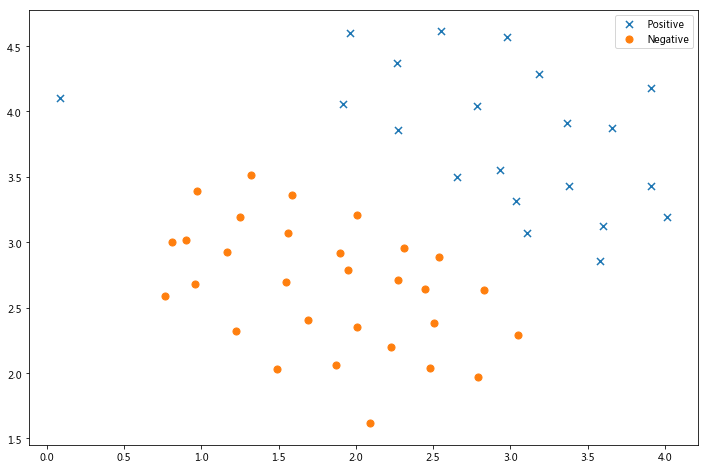
请注意，还有一个异常的正例在其他样本之外。
这些类仍然是线性分离的，但它非常紧凑。我们要训练线性支持向量机来学习类边界。

函数	作用
svc.decision_function(X)	样本X到分离超平面的距离
svc.fit(X, y[, sample_weight])	根据给定的训练数据拟合SVM模型。
svc.get_params([deep])	获取此估算器的参数并以字典行书储存,默认deep=True，以分类iris数据集为例，得到的参数如下
svc.predict(X)	根据测试数据集进行预测
svc.score(X, y[, sample_weight])	返回给定测试数据和标签的平均精确度
svc.predict_log_proba(X_test)，svc.predict_proba(X_test)	当sklearn.svm.SVC(probability=True)时，才会有这两个值，分别得到样本的对数概率以及普通概率。

令C=1

In [5]:

from sklearn import svm
svc = svm.LinearSVC(C=1, loss='hinge', max_iter=1000)
svc
'''
penalty : string, ‘l1’ or ‘l2’ (default=’l2’)

指定惩罚中使用的规范。 'l2'惩罚是SVC中使用的标准。 'l1'导致稀疏的coef_向量。

loss : string, ‘hinge’ or ‘squared_hinge’ (default=’squared_hinge’)

指定损失函数。 “hinge”是标准的SVM损失（例如由SVC类使用），而“squared_hinge”是hinge损失的平方。

dual : bool, (default=True)

选择算法以解决双优化或原始优化问题。 当n_samples> n_features时，首选dual = False。

tol : float, optional (default=1e-4)

公差停止标准

C : float, optional (default=1.0)

错误项的惩罚参数

multi_class : string, ‘ovr’ or ‘crammer_singer’ (default=’ovr’)

如果y包含两个以上的类，则确定多类策略。 “ovr”训练n_classes one-vs-rest分类器，而“crammer_singer”优化所有类的联合目标。 虽然crammer_singer在理论上是有趣的，因为它是一致的，但它在实践中很少使用，因为它很少能够提高准确性并且计算成本更高。 如果选择“crammer_singer”，则将忽略选项loss，penalty和dual。

fit_intercept : boolean, optional (default=True)

是否计算此模型的截距。 如果设置为false，则不会在计算中使用截距（即，预期数据已经居中）。

intercept_scaling : float, optional (default=1)

当self.fit_intercept为True时，实例向量x变为[x，self.intercept_scaling]，即具有等于intercept_scaling的常量值的“合成”特征被附加到实例向量。 截距变为intercept_scaling *合成特征权重注意！ 合成特征权重与所有其他特征一样经受l1 / l2正则化。 为了减小正则化对合成特征权重（并因此对截距）的影响，必须增加intercept_scaling。

class_weight : {dict, ‘balanced’}, optional

将类i的参数C设置为SVC的class_weight [i] * C. 如果没有给出，所有课程都应该有一个重量。 “平衡”模式使用y的值自动调整与输入数据中的类频率成反比的权重，如n_samples /（n_classes * np.bincount（y））

verbose : int, (default=0)

启用详细输出。 请注意，此设置利用liblinear中的每进程运行时设置，如果启用，可能无法在多线程上下文中正常工作。

random_state : int, RandomState instance or None, optional (default=None)

在随机数据混洗时使用的伪随机数生成器的种子。 如果是int，则random_state是随机数生成器使用的种子; 如果是RandomState实例，则random_state是随机数生成器; 如果为None，则随机数生成器是np.random使用的RandomState实例。

max_iter : int, (default=1000)

要运行的最大迭代次数。

'''

Out[5]:

LinearSVC(C=1, class_weight=None, dual=True, fit_intercept=True,
     intercept_scaling=1, loss='hinge', max_iter=1000, multi_class='ovr',
     penalty='l2', random_state=None, tol=0.0001, verbose=0)

In [6]:

svc.fit(data[['X1', 'X2']], data['y'])
svc.score(data[['X1', 'X2']], data['y'])
/opt/conda/lib/python3.6/site-packages/sklearn/svm/base.py:931: ConvergenceWarning: Liblinear failed to converge, increase the number of iterations.
  "the number of iterations.", ConvergenceWarning)

Out[6]:

0.9803921568627451

可视化分类边界

In [7]:

def find_decision_boundary(svc, x1min, x1max, x2min, x2max, diff):
    x1 = np.linspace(x1min, x1max, 1000)
    x2 = np.linspace(x2min, x2max, 1000)

    cordinates = [(x, y) for x in x1 for y in x2]
    x_cord, y_cord = zip(*cordinates)
    c_val = pd.DataFrame({'x1':x_cord, 'x2':y_cord})
    c_val['cval'] = svc.decision_function(c_val[['x1', 'x2']])

    decision = c_val[np.abs(c_val['cval']) < diff]
    
    return decision.x1, decision.x2

In [8]:

x1, x2 = find_decision_boundary(svc, 0, 4, 1.5, 5, 2 * 10**-3)
fig, ax = plt.subplots(figsize=(12,8))
ax.scatter(x1, x2, s=10, c='r',label='Boundary')
plot_init_data(data, fig, ax)
ax.set_title('SVM (C=1) Decision Boundary')
ax.legend()
plt.show()

其次，让我们看看如果C的值越大，会发生什么

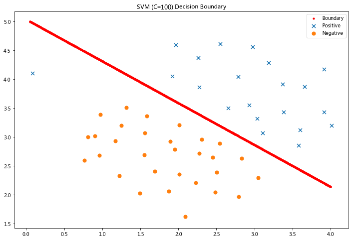
令C=100

In [9]:

svc2 = svm.LinearSVC(C=100, loss='hinge', max_iter=1000)
svc2.fit(data[['X1', 'X2']], data['y'])
svc2.score(data[['X1', 'X2']], data['y'])
/opt/conda/lib/python3.6/site-packages/sklearn/svm/base.py:931: ConvergenceWarning: Liblinear failed to converge, increase the number of iterations.
  "the number of iterations.", ConvergenceWarning)

Out[9]:

0.9019607843137255

这次我们得到了训练数据的完美分类，但是通过增加C的值，我们创建了一个不再适合数据的决策边界。我们可以通过查看每个类别预测的置信水平来看出这一点，这是该点与超平面距离的函数。

In [10]:

x1, x2 = find_decision_boundary(svc, 0, 4, 1.5, 5, 2 * 10**-3)
fig, ax = plt.subplots(figsize=(12,8))
ax.scatter(x1, x2, s=10, c='r',label='Boundary')
plot_init_data(data, fig, ax)
ax.set_title('SVM (C=100) Decision Boundary')
ax.legend()
plt.show()

1.1.1 线性内核

$θ^Tx^{(i)}=p^{(i)}\cdot{\left\| \theta \right\|}$

1.2 高斯内核的SVM

现在我们将从线性SVM转移到能够使用内核进行非线性分类的SVM。
虽然scikit-learn具有内置的高斯内核，但为了实现更清楚，我们将从头开始实现。

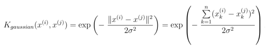
1.2.1 高斯内核

你把高斯内核认为是一个衡量一对数据间的“距离”的函数，有一个参数σ，决定了相似性下降至0有多快

Image Name

In [11]:

def gaussian_kernel(x1, x2, sigma):
    return np.exp(-(np.sum((x1 - x2) ** 2) / (2 * (sigma ** 2))))

In [12]:

x1 = np.array([1.0, 2.0, 1.0])
x2 = np.array([0.0, 4.0, -1.0])
sigma = 2

gaussian_kernel(x1, x2, sigma)

Out[12]:

0.32465246735834974

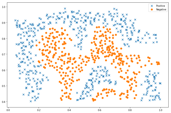
1.2.2 数据集2

接下来，我们在另一个数据集，上使高斯内核，找非线性边界。

In [13]:

raw_data = loadmat('/home/kesci/input/andrew_ml_ex67101/ex6data2.mat')

data = pd.DataFrame(raw_data['X'], columns=['X1', 'X2'])
data['y'] = raw_data['y']

fig, ax = plt.subplots(figsize=(12,8))
plot_init_data(data, fig, ax)
ax.legend()
plt.show()

In [14]:

svc = svm.SVC(C=100, gamma=10, probability=True)
svc

'''
C：C-SVC的惩罚参数C?默认值是1.0
C越大，相当于惩罚松弛变量，希望松弛变量接近0，即对误分类的惩罚增大，趋向于对训练集全分对的情况，这样对训练集测试时准确率很高，但泛化能力弱。C值小，对误分类的惩罚减小，允许容错，将他们当成噪声点，泛化能力较强。

kernel ：核函数，默认是rbf，可以是‘linear’, ‘poly’, ‘rbf’, ‘sigmoid’, ‘precomputed’
– 线性：u’v
– 多项式：(gamma*u’v + coef0)^degree
– RBF函数：exp(-gamma|u-v|^2)
–sigmoid：tanh(gammau’*v + coef0)

degree ：多项式poly函数的维度，默认是3，选择其他核函数时会被忽略。

gamma ： ‘rbf’,‘poly’ 和‘sigmoid’的核函数参数。默认是’auto’，则会选择1/n_features

coef0 ：核函数的常数项。对于‘poly’和 ‘sigmoid’有用。

probability ：是否采用概率估计.默认为False
布尔类型，可选，默认为False
决定是否启用概率估计。需要在训练fit()模型时加上这个参数，之后才能用相关的方法：predict_proba和predict_log_proba

shrinking ：是否采用shrinking heuristic方法，默认为true

tol ：停止训练的误差值大小，默认为1e-3

cache_size ：核函数cache缓存大小，默认为200

class_weight ：类别的权重，字典形式传递。设置第几类的参数C为weight*C(C-SVC中的C)

verbose ：允许冗余输出？

max_iter ：最大迭代次数。-1为无限制。

decision_function_shape ：‘ovo’, ‘ovr’ or None, default=None3

random_state ：数据洗牌时的种子值，int值
'''

Out[14]:

SVC(C=100, cache_size=200, class_weight=None, coef0=0.0,
  decision_function_shape='ovr', degree=3, gamma=10, kernel='rbf',
  max_iter=-1, probability=True, random_state=None, shrinking=True,
  tol=0.001, verbose=False)

In [15]:

svc.fit(data[['X1', 'X2']], data['y'])
svc.score(data[['X1', 'X2']], data['y'])

Out[15]:

0.9698725376593279

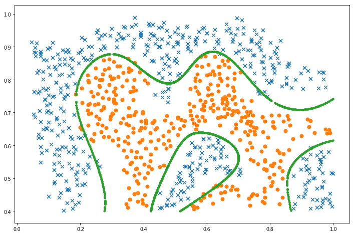
In [16]:

x1, x2 = find_decision_boundary(svc, 0, 1, 0.4, 1, 0.01)
fig, ax = plt.subplots(figsize=(12,8))
plot_init_data(data, fig, ax)
ax.scatter(x1, x2, s=10)
plt.show()

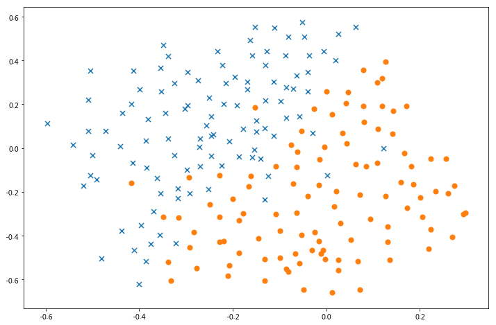
1.2.3 数据集3

对于第三个数据集，我们给出了训练和验证集，并且基于验证集性能为SVM模型找到最优超参数。
我们现在需要寻找最优C和σ，候选数值为[0.01, 0.03, 0.1, 0.3, 1, 3, 10, 30, 100]

In [17]:

raw_data = loadmat('/home/kesci/input/andrew_ml_ex67101/ex6data3.mat')

X = raw_data['X']
Xval = raw_data['Xval']
y = raw_data['y'].ravel()
yval = raw_data['yval'].ravel()

fig, ax = plt.subplots(figsize=(12,8))
data = pd.DataFrame(raw_data.get('X'), columns=['X1', 'X2'])
data['y'] = raw_data.get('y')
plot_init_data(data, fig, ax)
plt.show()

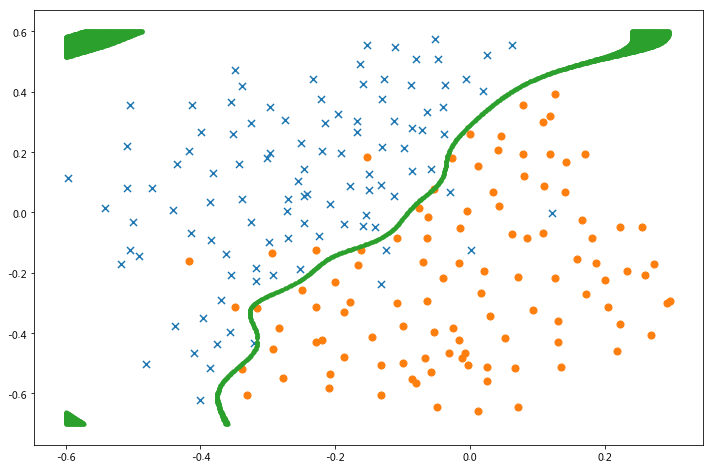
In [18]:

C_values = [0.01, 0.03, 0.1, 0.3, 1, 3, 10, 30, 100]
gamma_values = [0.01, 0.03, 0.1, 0.3, 1, 3, 10, 30, 100]

best_score = 0
best_params = {'C': None, 'gamma': None}

for C in C_values:
    for gamma in gamma_values:
        svc = svm.SVC(C=C, gamma=gamma)
        svc.fit(X, y)
        score = svc.score(Xval, yval)
        
        if score > best_score:
            best_score = score
            best_params['C'] = C
            best_params['gamma'] = gamma

best_score, best_params

Out[18]:

(0.965, {'C': 0.3, 'gamma': 100})

In [19]:

svc = svm.SVC(C=best_params['C'], gamma=best_params['gamma'])
svc.fit(X, y)

x1, x2 = find_decision_boundary(svc, -0.6, 0.3, -0.7, 0.6, 0.005)
fig, ax = plt.subplots(figsize=(12,8))
plot_init_data(data, fig, ax)
ax.scatter(x1, x2, s=10)
plt.show()

2 垃圾邮件分类

在这一部分中，我们的目标是使用SVM来构建垃圾邮件过滤器。

2.1 处理邮件

2.2 提取特征

这2个部分是处理邮件，以获得适合SVM处理的格式的数据。
然而，这个任务很简单（将字词映射到为练习提供的字典中的ID），而其余的预处理步骤（如HTML删除，词干，标准化等）已经完成。
我们就直接读取预先处理好的数据就可以了。

2.3 训练垃圾邮件分类SVM

In [20]:

spam_train = loadmat('/home/kesci/input/andrew_ml_ex67101/spamTrain.mat')
spam_test = loadmat('/home/kesci/input/andrew_ml_ex67101/spamTest.mat')

spam_train

Out[20]:

{'__header__': b'MATLAB 5.0 MAT-file, Platform: GLNXA64, Created on: Sun Nov 13 14:27:25 2011',
 '__version__': '1.0',
 '__globals__': [],
 'X': array([[0, 0, 0, ..., 0, 0, 0],
        [0, 0, 0, ..., 0, 0, 0],
        [0, 0, 0, ..., 0, 0, 0],
        ...,
        [0, 0, 0, ..., 0, 0, 0],
        [0, 0, 1, ..., 0, 0, 0],
        [0, 0, 0, ..., 0, 0, 0]], dtype=uint8),
 'y': array([[1],
        [1],
        [0],
        ...,
        [1],
        [0],
        [0]], dtype=uint8)}

In [21]:

X = spam_train['X']
Xtest = spam_test['Xtest']
y = spam_train['y'].ravel()
ytest = spam_test['ytest'].ravel()

X.shape, y.shape, Xtest.shape, ytest.shape

Out[21]:

((4000, 1899), (4000,), (1000, 1899), (1000,))

每个文档已经转换为一个向量，其中1,899个维对应于词汇表中的1,899个单词。它们的值为二进制，表示文档中是否存在单词。

In [22]:

svc = svm.SVC()
svc.fit(X, y)
/opt/conda/lib/python3.6/site-packages/sklearn/svm/base.py:196: FutureWarning: The default value of gamma will change from 'auto' to 'scale' in version 0.22 to account better for unscaled features. Set gamma explicitly to 'auto' or 'scale' to avoid this warning.
  "avoid this warning.", FutureWarning)

Out[22]:

SVC(C=1.0, cache_size=200, class_weight=None, coef0=0.0,
  decision_function_shape='ovr', degree=3, gamma='auto_deprecated',
  kernel='rbf', max_iter=-1, probability=False, random_state=None,
  shrinking=True, tol=0.001, verbose=False)

In [23]:

print('Training accuracy = {0}%'.format(np.round(svc.score(X, y) * 100, 2)))
print('Test accuracy = {0}%'.format(np.round(svc.score(Xtest, ytest) * 100, 2)))
Training accuracy = 94.4%
Test accuracy = 95.3%

2.4 可视化结果

In [24]:

kw = np.eye(1899)
kw[:3,:]
spam_val = pd.DataFrame({'idx':range(1899)})

In [25]:

spam_val['isspam'] = svc.decision_function(kw)

In [26]:

spam_val['isspam'].describe()

Out[26]:

count    1899.000000
mean       -0.622564
std         0.021603
min        -0.763138
25%        -0.631616
50%        -0.624299
75%        -0.615918
max        -0.364164
Name: isspam, dtype: float64

In [27]:

decision = spam_val[spam_val['isspam'] > -0.55]
decision

Out[27]:

	idx	isspam
173	173	-0.546054
297	297	-0.364164
478	478	-0.543913
529	529	-0.524535
680	680	-0.524313
738	738	-0.549962
774	774	-0.489291
1059	1059	-0.547064
1088	1088	-0.531602
1163	1163	-0.549382
1190	1190	-0.420982
1263	1263	-0.476572
1372	1372	-0.527429
1397	1397	-0.432722
1818	1818	-0.517247
1851	1851	-0.536655
1892	1892	-0.511805
1894	1894	-0.458944

In [28]:

path =  '/home/kesci/input/andrew_ml_ex67101/vocab.txt'
voc = pd.read_csv(path, header=None, names=['idx', 'voc'], sep = '\t')
voc.head()

Out[28]:

	idx	voc
0	1	aa
1	2	ab
2	3	abil
3	4	abl
4	5	about

In [29]:

spamvoc = voc.loc[list(decision['idx'])]
spamvoc

sOut[29]:

	idx	voc
173	174	below
297	298	click
478	479	dollarnumb
529	530	email
680	681	free
738	739	guarante
774	775	here
1059	1060	monei
1088	1089	nbsp
1163	1164	offer
1190	1191	our
1263	1264	pleas
1372	1373	receiv
1397	1398	remov
1818	1819	we
1851	1852	will
1892	1893	you