CPT204 Advanced Obejct-Oriented Programming 高级面向对象编程 Pt.9 图-CSDN博客

本文链接：https://blog.csdn.net/sensen_kiss/article/details/147700118

1. 图

1.1 图的基础知识

我们在算法和数学中都学习过图。
图是一种强大的工具，可以将复杂的现实世界问题抽象化，通过节点（vertices）和边（edges）来表示对象及其关系，从而更容易理解和解决问题。
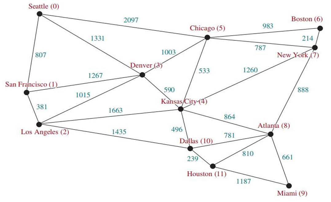
其经常的应用是分析城市间的最短路径，更清晰地表达是寻找两个城市之间最少航班的问题，可以转化为在图中找到两个顶点之间的最短路径。也可以用于社交媒体分析（建模社交网络）、计算机芯片设计、搜索引擎算法。

图 $G = (V, E)$
图 $G$ 是由两个集合组成的数学结构：
$V$ 表示顶点集合（Vertices 或 Nodes），是一组离散的对象。
$E$ 表示边集合（Edges 或 Links），是一组连接顶点的连接关系。
无向图（Undirected Graph）是一种图，其中的边没有方向。在无向图中，边 $(x, y)$ 和 $边 (y, x)$ 是相同的，因为它们表示的是同一个连接关系。
有向图（Directed Graph，也称为“有向图”或“Digraph”）是一种图，其中的边有方向。在有向图中，边 $(x, y)$ 和边 $(y, x)$ 是不同的，因为它们的方向不同。

如果两个顶点通过一条边连接，那么这两个顶点被称为相邻的（Adjacent）或邻居（Neighbors）。
连接两个顶点的边被称为与这两个顶点相关联的（Incident）。
如图中 $A$ 和 $B$ 是相邻的。
在这里插入图片描述
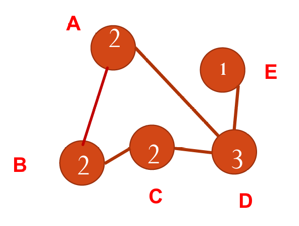
度（Degree）：一个顶点的度是指与该顶点相关联的边的数量。
对于无向图，顶点的度就是与它相连的边的数量。例如，如果一个顶点与三条边相连，那么它的度就是3。
对于有向图，顶点的度分为入度（In-degree）和出度（Out-degree）：
入度（In-degree）：指向该顶点的边的数量。
出度（Out-degree）：从该顶点出发的边的数量。
顶点的总度数是入度和出度之和。
下图给出了关于度的无向图例子。
在这里插入图片描述

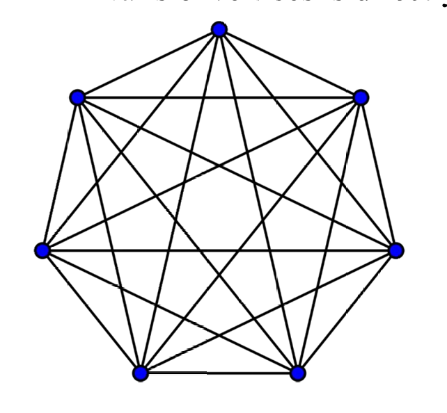
完全图是一种图，其中每一对不同的顶点之间都有一条边直接相连。在完全图中，每个顶点的度都等于顶点总数减一（因为一个顶点不能与自己相连）。
如下图所示。
在这里插入图片描述

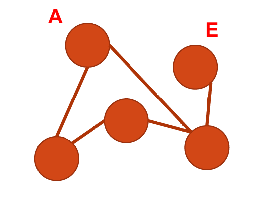
不完全图是一种图，其中至少存在一对顶点之间没有直接的边相连。
如下图所示， $A$ 、 $E$ 之间没有直接的边相连。
在这里插入图片描述

在无权图（Unweighted）中，边没有与它们关联的权重（weight）。换句话说，图中的所有边都被认为具有相同的“成本”或“距离”。如前面的图都是无权图。
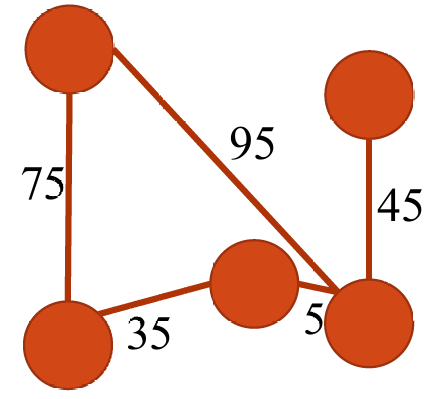
在加权图（Weighted）中，每条边都有一个与之关联的权重，这个权重可以代表成本、距离、时间或其他任何可以量化的度量。
如下图所示。
在这里插入图片描述

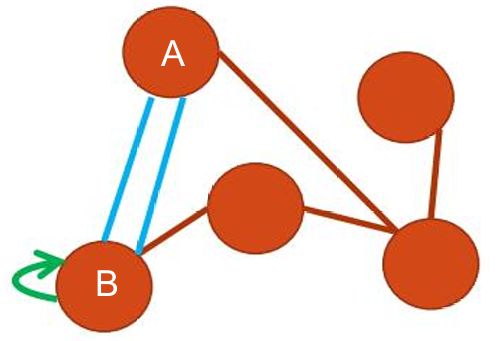
如果两个顶点之间存在两条或多条边，这些边被称为平行边（Parallel Edges）。
环（Loops）是一种特殊的边，它将一个顶点直接连接到它自己。
简单图（Simple Graph）是一种特殊的图，它不包含任何平行边或环。
下图不是一个简单图，因为他有平行边，也有环，而前面的图都是简单图。
在这里插入图片描述
闭合路径（Closed Path）是一种路径，其中所有顶点都恰好有两条边与之相关联（即每个顶点的度数为2）。
闭合路径是一条从某个顶点出发，经过一系列其他顶点后，最终回到起始顶点的路径。在闭合路径中，除了起始和结束顶点外，其他所有顶点都恰好连接两条边，这两条边分别指向路径的前后两个顶点。
环（Cycle）是一种特殊的闭合路径，它从同一个顶点开始并在同一个顶点结束。
环是一条起点和终点相同的路径，它不包含重复的边，除非起点和终点是同一个顶点。环的长度至少为3（即至少包含三个顶点），因为至少需要三个顶点才能形成一个环（一个顶点到自己的环没有实际意义）。

如果图中任意两个顶点之间都存在至少一条路径，那么这个图被称为连通图（Connected Graph）。
前面展示的图都是连通图。

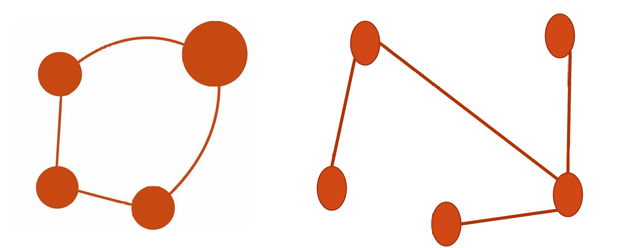
树是一种特殊的连通图，它满足以下两个条件：

连通性：图中任意两个顶点之间都存在至少一条路径，即图是连通的。
无环性：图中不包含任何环，即不存在从某个顶点出发，沿着边走能够回到起始顶点的路径（除了顶点自身形成的自环，但树中不允许有自环）。

下图左侧不是树，因为有环存在，右侧是。
在这里插入图片描述

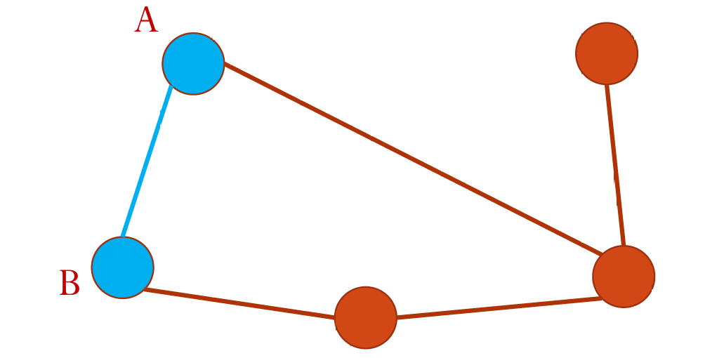
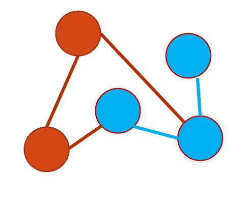
子图（Subgraph）是从一个更大的图（称为原图或超图）中通过选择一部分顶点和边而形成的新图。
如下图所示，这里红色的部分或者蓝色的部分都是整个图的子图。
在这里插入图片描述

1.2 图的表示。

图（Graphs）在计算机科学中常见的几种数据结构表示方法如下：
顶点可以用简单的数据结构（如数组、列表或哈希表）来表示，其中每个顶点都有一个唯一的标识符。
边的表示方式有很多：

边数组（Edge Array），使用数组来存储图中所有边。
边对象（Edge Objects），使用对象来表示每条边。
邻接矩阵（Adjacency Matrices），使用二维数组来表示图中顶点之间连接关系。
邻接表（Adjacency Lists），使用列表来表示图中每个顶点的邻接顶点或者邻接边。

1.2.1 顶点的表示

使用数组表示顶点的例子如下：

String[] vertices = {"Seattle", "San Francisco", "Los Angeles", "Denver", "Kansas City", /* ... */};

使用列表表示顶点的例子如下：

List<String> vertices;
vertices.add("Seattle");

使用对象的方法也可以，例子如下：

public class City {
    // 定义属性，例如城市名称
    private String cityName;

    // 定义构造函数
    public City(String cityName) {
        this.cityName = cityName;
    }

    // 定义获取城市名称的方法
    public String getCityName() {
        return cityName;
    }

    // 定义设置城市名称的方法
    public void setCityName(String cityName) {
        this.cityName = cityName;
    }
}

// 创建City类的实例
City city0 = new City("Seattle");
City city1 = new City("San Francisco");

// 使用City类的实例创建数组
City[] vertices = {city0, city1, /* ... */};

1.2.2 边的表示

1.2.2.1 边数组

我们可以使用使用二维数组表示边（Edge Array），例子如下。

int[][] edges = {        
    {0, 1}, {0, 3}, {0, 5}, // 从顶点 0 出发的边
    {1, 0}, {1, 2}, {1, 3}, // 从顶点 1 出发的边
    {2, 1}, {2, 3}, {2, 4}, {2, 10},
    {3, 0}, {3, 1}, {3, 2}, {3, 4}, {3, 5},
    {4, 2}, {4, 3}, {4, 5}, {4, 7}, {4, 8}, {4, 10}, 
    {5, 0}, {5, 3}, {5, 4}, {5, 6}, {5, 7},
    {6, 5}, {6, 7}, // 后续边...
};

每对数字，例如 {0, 1}，表示从顶点 0 到顶点 1 存在一条边。
在无权图中，边没有权重，因此 {0, 1} 和 {1, 0} 表示的是同一条边。

1.2.2.2 边对象

我们可以使用边对象（Edge Objects）来表示图中的边，例子如下。

public class Edge {
    // 定义边的两个端点
    int u, v;

    // 构造函数
    public Edge(int u, int v) {
        this.u = u;
        this.v = v;
    }

    // getter 和 setter 方法
    public int getU() {
        return u;
    }

    public void setU(int u) {
        this.u = u;
    }

    public int getV() {
        return v;
    }

    public void setV(int v) {
        this.v = v;
    }
}

// 创建一个 ArrayList 来存储边对象
List<Edge> list = new ArrayList<>();
list.add(new Edge(0, 1));
list.add(new Edge(0, 3));

使用 ArrayList 存储边对象的一个主要优势是其动态性。你不需要事先知道图中边的数量，可以随着需要动态地添加边对象。

1.2.2.3 邻接矩阵

我们可以使用邻接矩阵表示边（Adjacency Matrix），例子如下。

int[][] adjacencyMatrix = {
    {0, 1, 0, 1}, // 西雅图（Seattle）
    {1, 0, 1, 1}, // 旧金山（San Francisco）
    {0, 1, 0, 1}, // 洛杉矶（Los Angeles）
    {1, 1, 1, 0}, // 丹佛（Denver）
};

在这里插入图片描述

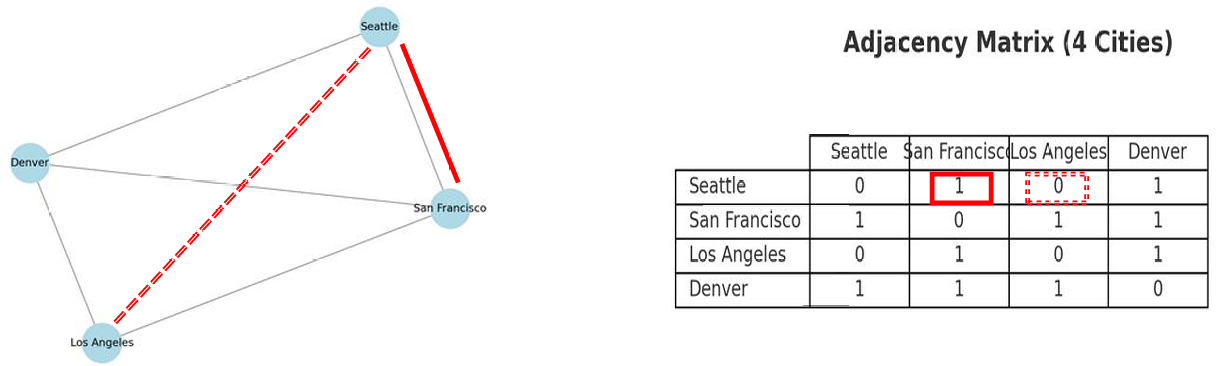
矩阵中的每个元素[i,j]表示从顶点 i 到顶点 j 是否存在边。

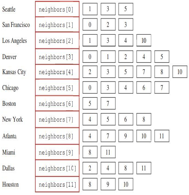
1.2.2.4 邻接顶点列表（Adjacency Vertex List）

我们可以使用邻接顶点列表（Adjacency Vertex List）来表示图中的边，例子如下。

// 创建一个包含12个整数列表的数组，每个列表代表一个城市
List<Integer>[] neighbors = new List[12];

// 向每个城市的邻居列表中添加整数（即城市索引），表示与当前城市相连的邻近城市
neighbors[0].add(1); // 旧金山（San Francisco）与索引为1的城市相邻
neighbors[0].add(3); // 旧金山（San Francisco）与索引为3的城市相邻
neighbors[0].add(5); // 旧金山（San Francisco）与索引为5的城市相邻

neighbors[1].add(0); // 西雅图（Seattle）与索引为0的城市相邻
neighbors[1].add(2); // 西雅图（Seattle）与索引为2的城市相邻
neighbors[1].add(3); // 西雅图（Seattle）与索引为3的城市相邻

邻接顶点列表是一种使用数组来存储每个顶点的邻接顶点的表示方法。每个顶点对应一个列表，列表中包含与该顶点直接相连的所有顶点的索引。
在这里插入图片描述

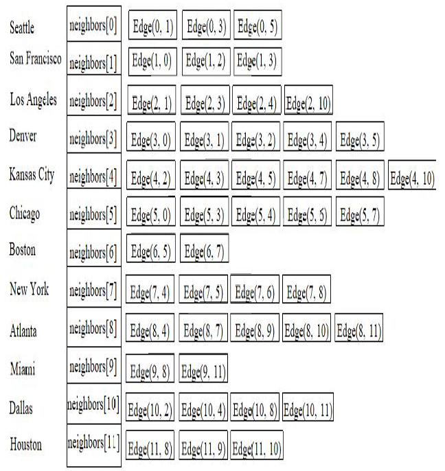
1.2.2.5 邻接边列表（Adjacency Edge List）

与邻接顶点列表不同，邻接边列表存储的是边对象（Edge Objects）而不是顶点索引。
因此需要定义边对象。

public class Edge {
    int u; // 边的起点顶点
    int v; // 边的终点顶点

    // 构造函数，用于初始化边的起点和终点
    public Edge(int u, int v) {
        this.u = u;
        this.v = v;
    }
}

然后使用邻接边列表表示边。

// 创建一个包含12个边对象列表的数组，每个列表代表一个顶点的邻接边
List<Edge>[] neighbors = new List[12];

// 向每个顶点的邻接边列表中添加边对象，表示与当前顶点相连的边
neighbors[0].add(new Edge(0, 1));  // 西雅图（Seattle）到旧金山（San Francisco）
neighbors[0].add(new Edge(0, 3));  // 西雅图（Seattle）到丹佛（Denver）
neighbors[0].add(new Edge(0, 5));  // 西雅图（Seattle）到芝加哥（Chicago）

在这里插入图片描述

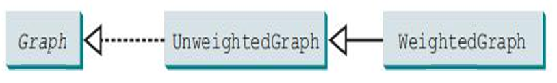
1.3 对图建模

我们现在准备对图进行建模。我们会创建一个名为 Graph 的接口，该接口包含所有图的通用操作。然后是UnweightedGraph 和 WeightedGraph 类，它们实现了 Graph 接口。这些类定义了内部数据结构来存储图的信息，例如使用邻接表（Adjacency List）或邻接矩阵（Adjacency Matrix）来表示图的顶点和边。为了让用户能够从不同类型的输入初始化图，这些类提供了多个构造函数。这些类通过提供具体逻辑来实现 Graph 接口中声明的抽象方法。
在这里插入图片描述
代码如下。

public interface Graph<V> {
    /**
     * Return the number of vertices in the graph
     */
    public int getSize();

    /**
     * Return the vertices in the graph
     */
    public java.util.List<V> getVertices();

    /**
     * Return the object for the specified vertex index
     */
    public V getVertex(int index);

    /**
     * Return the index for the specified vertex object
     */
    public int getIndex(V v);

    /**
     * Return the neighbors of vertex with the specified index
     */
    public java.util.List<Integer> getNeighbors(int index);

    /**
     * Return the degree for a specified vertex
     */
    public int getDegree(int v);

    /**
     * Print the edges
     */
    public void printEdges();

    /**
     * Clear the graph
     */
    public void clear();

    /**
     * Add a vertex to the graph
     */
    public boolean addVertex(V vertex);

    /**
     * Add an edge (u, v) to the graph
     */
    public boolean addEdge(int u, int v);

    /**
     * Add an edge to the graph
     */
    public boolean addEdge(Edge e);

    /**
     * Remove a vertex v from the graph, return true if successful
     */
    public boolean remove(V v);

    /**
     * Remove an edge (u, v) from the graph
     */
    public boolean remove(int u, int v);

    /**
     * Obtain a depth-first search tree
     */
    public UnweightedGraph<V>.SearchTree dfs(int v);

    /**
     * Obtain a breadth-first search tree
     */
    public UnweightedGraph<V>.SearchTree bfs(int v);
}

UnweightedGraph类的代码如下。

import java.util.*;

public class UnweightedGraph<V> implements Graph<V> {
    protected List<V> vertices = new ArrayList<>(); // Store vertices
    protected List<List<Edge>> neighbors
            = new ArrayList<>(); // Adjacency lists

    /**
     * Construct an empty graph
     */
    public UnweightedGraph() {
    }

    /**
     * Construct a graph from vertices and edges stored in arrays
     */
    public UnweightedGraph(V[] vertices, int[][] edges) {
        for (int i = 0; i < vertices.length; i++)
            addVertex(vertices[i]);

        createAdjacencyLists(edges, vertices.length);
    }

    /**
     * Construct a graph from vertices and edges stored in List
     */
    public UnweightedGraph(List<V> vertices, List<Edge> edges) {
        for (int i = 0; i < vertices.size(); i++)
            addVertex(vertices.get(i));

        createAdjacencyLists(edges, vertices.size());
    }

    /**
     * Construct a graph for integer vertices 0, 1, 2 and edge list
     */
    public UnweightedGraph(List<Edge> edges, int numberOfVertices) {
        for (int i = 0; i < numberOfVertices; i++)
            addVertex((V) (new Integer(i))); // vertices is {0, 1, ...}

        createAdjacencyLists(edges, numberOfVertices);
    }

    /**
     * Construct a graph from integer vertices 0, 1, and edge array
     */
    public UnweightedGraph(int[][] edges, int numberOfVertices) {
        for (int i = 0; i < numberOfVertices; i++)
            addVertex((V) (new Integer(i))); // vertices is {0, 1, ...}

        createAdjacencyLists(edges, numberOfVertices);
    }

    /**
     * Create adjacency lists for each vertex
     */
    private void createAdjacencyLists(
            int[][] edges, int numberOfVertices) {
        for (int i = 0; i < edges.length; i++) {
            addEdge(edges[i][0], edges[i][1]);
        }
    }

    /**
     * Create adjacency lists for each vertex
     */
    private void createAdjacencyLists(
            List<Edge> edges, int numberOfVertices) {
        for (Edge edge : edges) {
            addEdge(edge.u, edge.v);
        }
    }

    @Override
    /** Return the number of vertices in the graph */
    public int getSize() {
        return vertices.size();
    }

    @Override
    /** Return the vertices in the graph */
    public List<V> getVertices() {
        return vertices;
    }

    @Override
    /** Return the object for the specified vertex */
    public V getVertex(int index) {
        return vertices.get(index);
    }

    @Override
    /** Return the index for the specified vertex object */
    public int getIndex(V v) {
        return vertices.indexOf(v);
    }

    @Override
    /** Return the neighbors of the specified vertex */
    public List<Integer> getNeighbors(int index) {
        List<Integer> result = new ArrayList<>();
        for (Edge e : neighbors.get(index))
            result.add(e.v);

        return result;
    }

    @Override
    /** Return the degree for a specified vertex */
    public int getDegree(int v) {
        return neighbors.get(v).size();
    }

    @Override
    /** Print the edges */
    public void printEdges() {
        for (int u = 0; u < neighbors.size(); u++) {
            System.out.print(getVertex(u) + " (" + u + "): ");
            for (Edge e : neighbors.get(u)) {
                System.out.print("(" + getVertex(e.u) + ", " +
                        getVertex(e.v) + ") ");
            }
            System.out.println();
        }
    }

    @Override
    /** Clear the graph */
    public void clear() {
        vertices.clear();
        neighbors.clear();
    }

    @Override
    /** Add a vertex to the graph */
    public boolean addVertex(V vertex) {
        if (!vertices.contains(vertex)) {
            vertices.add(vertex);
            neighbors.add(new ArrayList<Edge>());
            return true;
        } else {
            return false;
        }
    }

    @Override
    /** Add an edge to the graph */
    public boolean addEdge(Edge e) {
        if (e.u < 0 || e.u > getSize() - 1)
            throw new IllegalArgumentException("No such index: " + e.u);

        if (e.v < 0 || e.v > getSize() - 1)
            throw new IllegalArgumentException("No such index: " + e.v);

        if (!neighbors.get(e.u).contains(e)) {
            neighbors.get(e.u).add(e);
            return true;
        } else {
            return false;
        }
    }

    @Override
    /** Add an edge to the graph */
    public boolean addEdge(int u, int v) {
        return addEdge(new Edge(u, v));
    }

    @Override
    /** Obtain a DFS tree starting from vertex u */
    /** To be discussed in Section 28.7 */
    public SearchTree dfs(int v) {
        List<Integer> searchOrder = new ArrayList<>();
        int[] parent = new int[vertices.size()];
        for (int i = 0; i < parent.length; i++)
            parent[i] = -1; // Initialize parent[i] to -1

        // Mark visited vertices
        boolean[] isVisited = new boolean[vertices.size()];

        // Recursively search
        dfs(v, parent, searchOrder, isVisited);

        // Return a search tree
        return new SearchTree(v, parent, searchOrder);
    }

    /**
     * Recursive method for DFS search
     */
    private void dfs(int v, int[] parent, List<Integer> searchOrder,
                     boolean[] isVisited) {
        // Store the visited vertex
        searchOrder.add(v);
        isVisited[v] = true; // Vertex v visited

        for (Edge e : neighbors.get(v)) { // Note that e.u is v
            if (!isVisited[e.v]) { // e.v is w in Listing 28.8
                parent[e.v] = v; // The parent of w is v
                dfs(e.v, parent, searchOrder, isVisited); // Recursive search
            }
        }
    }

    @Override
    /** Starting bfs search from vertex v */
    /** To be discussed in Section 28.9 */
    public SearchTree bfs(int v) {
        List<Integer> searchOrder = new ArrayList<>();
        int[] parent = new int[vertices.size()];
        for (int i = 0; i < parent.length; i++)
            parent[i] = -1; // Initialize parent[i] to -1

        java.util.LinkedList<Integer> queue =
                new java.util.LinkedList<>(); // list used as a queue
        boolean[] isVisited = new boolean[vertices.size()];
        queue.offer(v); // Enqueue v
        isVisited[v] = true; // Mark it visited

        while (!queue.isEmpty()) {
            int u = queue.poll(); // Dequeue to u
            searchOrder.add(u); // u searched
            for (Edge e : neighbors.get(u)) { // Note that e.u is u
                if (!isVisited[e.v]) { // e.v is w in Listing 28.11
                    queue.offer(e.v); // Enqueue w
                    parent[e.v] = u; // The parent of w is u
                    isVisited[e.v] = true; // Mark w visited
                }
            }
        }

        return new SearchTree(v, parent, searchOrder);
    }

    /** Tree inner class inside the UnweightedGraph class */
    /**
     * To be discussed in Section 28.6
     */
    public class SearchTree {
        private int root; // The root of the tree
        private int[] parent; // Store the parent of each vertex
        private List<Integer> searchOrder; // Store the search order

        /**
         * Construct a tree with root, parent, and searchOrder
         */
        public SearchTree(int root, int[] parent,
                          List<Integer> searchOrder) {
            this.root = root;
            this.parent = parent;
            this.searchOrder = searchOrder;
        }

        /**
         * Return the root of the tree
         */
        public int getRoot() {
            return root;
        }

        /**
         * Return the parent of vertex v
         */
        public int getParent(int v) {
            return parent[v];
        }

        /**
         * Return an array representing search order
         */
        public List<Integer> getSearchOrder() {
            return searchOrder;
        }

        /**
         * Return number of vertices found
         */
        public int getNumberOfVerticesFound() {
            return searchOrder.size();
        }

        /**
         * Return the path of vertices from a vertex to the root
         */
        public List<V> getPath(int index) {
            ArrayList<V> path = new ArrayList<>();

            do {
                path.add(vertices.get(index));
                index = parent[index];
            }
            while (index != -1);

            return path;
        }

        /**
         * Print a path from the root to vertex v
         */
        public void printPath(int index) {
            List<V> path = getPath(index);
            System.out.print("A path from " + vertices.get(root) + " to " +
                    vertices.get(index) + ": ");
            for (int i = path.size() - 1; i >= 0; i--)
                System.out.print(path.get(i) + " ");
        }

        /**
         * Print the whole tree
         */
        public void printTree() {
            System.out.println("Root is: " + vertices.get(root));
            System.out.print("Edges: ");
            for (int i = 0; i < parent.length; i++) {
                if (parent[i] != -1) {
                    // Display an edge
                    System.out.print("(" + vertices.get(parent[i]) + ", " +
                            vertices.get(i) + ") ");
                }
            }
            System.out.println();
        }
    }

    @Override
    /** Remove vertex v and return true if successful */
    public boolean remove(V v) {
        return true; // Implementation left as an exercise
    }

    @Override
    /** Remove edge (u, v) and return true if successful */
    public boolean remove(int u, int v) {
        return true; // Implementation left as an exercise
    }
}

WeightedGraph类的代码如下。

import java.util.*;

public class WeightedGraph<V> extends UnweightedGraph<V> {
    /**
     * Construct an empty
     */
    public WeightedGraph() {
    }

    /**
     * Construct a WeightedGraph from vertices and edged in arrays
     */
    public WeightedGraph(V[] vertices, int[][] edges) {
        createWeightedGraph(java.util.Arrays.asList(vertices), edges);
    }

    /**
     * Construct a WeightedGraph from vertices and edges in list
     */
    public WeightedGraph(int[][] edges, int numberOfVertices) {
        List<V> vertices = new ArrayList<>();
        for (int i = 0; i < numberOfVertices; i++)
            vertices.add((V) (new Integer(i)));

        createWeightedGraph(vertices, edges);
    }

    /**
     * Construct a WeightedGraph for vertices 0, 1, 2 and edge list
     */
    public WeightedGraph(List<V> vertices, List<WeightedEdge> edges) {
        createWeightedGraph(vertices, edges);
    }

    /**
     * Construct a WeightedGraph from vertices 0, 1, and edge array
     */
    public WeightedGraph(List<WeightedEdge> edges,
                         int numberOfVertices) {
        List<V> vertices = new ArrayList<>();
        for (int i = 0; i < numberOfVertices; i++)
            vertices.add((V) (new Integer(i)));

        createWeightedGraph(vertices, edges);
    }

    /**
     * Create adjacency lists from edge arrays
     */
    private void createWeightedGraph(List<V> vertices, int[][] edges) {
        this.vertices = vertices;

        for (int i = 0; i < vertices.size(); i++) {
            neighbors.add(new ArrayList<Edge>()); // Create a list for vertices
        }

        for (int i = 0; i < edges.length; i++) {
            neighbors.get(edges[i][0]).add(
                    new WeightedEdge(edges[i][0], edges[i][1], edges[i][2]));
        }
    }

    /**
     * Create adjacency lists from edge lists
     */
    private void createWeightedGraph(
            List<V> vertices, List<WeightedEdge> edges) {
        this.vertices = vertices;

        for (int i = 0; i < vertices.size(); i++) {
            neighbors.add(new ArrayList<Edge>()); // Create a list for vertices
        }

        for (WeightedEdge edge : edges) {
            neighbors.get(edge.u).add(edge); // Add an edge into the list
        }
    }

    /**
     * Return the weight on the edge (u, v)
     */
    public double getWeight(int u, int v) throws Exception {
        for (Edge edge : neighbors.get(u)) {
            if (edge.v == v) {
                return ((WeightedEdge) edge).weight;
            }
        }

        throw new Exception("Edge does not exit");
    }

    /**
     * Display edges with weights
     */
    public void printWeightedEdges() {
        for (int i = 0; i < getSize(); i++) {
            System.out.print(getVertex(i) + " (" + i + "): ");
            for (Edge edge : neighbors.get(i)) {
                System.out.print("(" + edge.u +
                        ", " + edge.v + ", " + ((WeightedEdge) edge).weight + ") ");
            }
            System.out.println();
        }
    }

    /**
     * Add an edge (u, v, weight) to the graph.
     */
    public boolean addEdge(int u, int v, double weight) {
        return addEdge(new WeightedEdge(u, v, weight));
    }

    /**
     * Get a minimum spanning tree rooted at vertex 0
     */
    public MST getMinimumSpanningTree() {
        return getMinimumSpanningTree(0);
    }

    /**
     * Get a minimum spanning tree rooted at a specified vertex
     */
    public MST getMinimumSpanningTree(int startingVertex) {
        // cost[v] stores the cost by adding v to the tree
        double[] cost = new double[getSize()];
        for (int i = 0; i < cost.length; i++) {
            cost[i] = Double.POSITIVE_INFINITY; // Initial cost
        }
        cost[startingVertex] = 0; // Cost of source is 0

        int[] parent = new int[getSize()]; // Parent of a vertex
        parent[startingVertex] = -1; // startingVertex is the root
        double totalWeight = 0; // Total weight of the tree thus far

        List<Integer> T = new ArrayList<>();

        // Expand T
        while (T.size() < getSize()) {
            // Find smallest cost u in V - T
            int u = -1; // Vertex to be determined
            double currentMinCost = Double.POSITIVE_INFINITY;
            for (int i = 0; i < getSize(); i++) {
                if (!T.contains(i) && cost[i] < currentMinCost) {
                    currentMinCost = cost[i];
                    u = i;
                }
            }

            if (u == -1) break;
            else T.add(u); // Add a new vertex to T
            totalWeight += cost[u]; // Add cost[u] to the tree

            // Adjust cost[v] for v that is adjacent to u and v in V - T
            for (Edge e : neighbors.get(u)) {
                if (!T.contains(e.v) && cost[e.v] > ((WeightedEdge) e).weight) {
                    cost[e.v] = ((WeightedEdge) e).weight;
                    parent[e.v] = u;
                }
            }
        }

        return new MST(startingVertex, parent, T, totalWeight);
    }

    /**
     * MST is an inner class in WeightedGraph
     */
    public class MST extends SearchTree {
        private double totalWeight; // Total weight of all edges in the tree

        public MST(int root, int[] parent, List<Integer> searchOrder,
                   double totalWeight) {
            super(root, parent, searchOrder);
            this.totalWeight = totalWeight;
        }

        public double getTotalWeight() {
            return totalWeight;
        }
    }

    /**
     * Find single source shortest paths
     */
    public ShortestPathTree getShortestPath(int sourceVertex) {
        // cost[v] stores the cost of the path from v to the source
        double[] cost = new double[getSize()];
        for (int i = 0; i < cost.length; i++) {
            cost[i] = Double.POSITIVE_INFINITY; // Initial cost set to infinity
        }
        cost[sourceVertex] = 0; // Cost of source is 0

        // parent[v] stores the previous vertex of v in the path
        int[] parent = new int[getSize()];
        parent[sourceVertex] = -1; // The parent of source is set to -1

        // T stores the vertices whose path found so far
        List<Integer> T = new ArrayList<>();

        // Expand T
        while (T.size() < getSize()) {
            // Find smallest cost v in V - T
            int u = -1; // Vertex to be determined
            double currentMinCost = Double.POSITIVE_INFINITY;
            for (int i = 0; i < getSize(); i++) {
                if (!T.contains(i) && cost[i] < currentMinCost) {
                    currentMinCost = cost[i];
                    u = i;
                }
            }

            if (u == -1) break;
            else T.add(u); // Add a new vertex to T

            // Adjust cost[v] for v that is adjacent to u and v in V - T
            for (Edge e : neighbors.get(u)) {
                if (!T.contains(e.v)
                        && cost[e.v] > cost[u] + ((WeightedEdge) e).weight) {
                    cost[e.v] = cost[u] + ((WeightedEdge) e).weight;
                    parent[e.v] = u;
                }
            }
        } // End of while

        // Create a ShortestPathTree
        return new ShortestPathTree(sourceVertex, parent, T, cost);
    }

    /**
     * ShortestPathTree is an inner class in WeightedGraph
     */
    public class ShortestPathTree extends SearchTree {
        private double[] cost; // cost[v] is the cost from v to source

        /**
         * Construct a path
         */
        public ShortestPathTree(int source, int[] parent,
                                List<Integer> searchOrder, double[] cost) {
            super(source, parent, searchOrder);
            this.cost = cost;
        }

        /**
         * Return the cost for a path from the root to vertex v
         */
        public double getCost(int v) {
            return cost[v];
        }

        /**
         * Print paths from all vertices to the source
         */
        public void printAllPaths() {
            System.out.println("All shortest paths from " +
                    vertices.get(getRoot()) + " are:");
            for (int i = 0; i < cost.length; i++) {
                printPath(i); // Print a path from i to the source
                System.out.println("(cost: " + cost[i] + ")"); // Path cost
            }
        }
    }
}

1.3.1 图遍历（以无权图为例）

这里面还涉及了其他的一些内容，比如图遍历算法。图遍历是指按照某种顺序访问图中的每个顶点，且每个顶点仅被访问一次的过程。
常见的两种方法是深度优先搜索（Depth-First Search, DFS）和广度优先搜索（Breadth-First Search, BFS），无论是 DFS 还是 BFS，遍历图的过程都会生成一个生成树（Spanning Tree），这是原图的一个子图，包含了图中的所有顶点。

1.3.1.1 深度优先搜索（Depth-First Search, DFS）

DFS 从图中的某个顶点开始，尽可能深地搜索图的分支，直到不能继续为止，然后回溯。
具体步骤如下：

访问当前顶点：标记当前顶点 $v$ 为已访问。
遍历邻居：对于 $v$ 的每个邻居 $w$ ：
如果 $w$ 未被访问：
在搜索树中将 $v$ 设置为 $w$ 的父顶点。
递归地访问 $w$ ，这将在每次递归步骤中改变当前顶点。

伪代码如下。

Tree dfs(vertex v) {
    // 标记当前顶点为已访问
    visit(v);
    // 遍历每个邻居
    for each neighbor w of v {
        // 如果这个邻居未被访问
        if (w has not been visited) {
            // 在搜索树中将 v 设置为 w 的父顶点
            set v as the parent for w;
            // 递归地访问 w
            dfs(w);
        }
    }
}

它的时间复杂度为 $O (∣ E ∣ + ∣ V ∣)$
由于每个顶点恰好被访问一次，因此与顶点相关的操作总数是 $∣ V ∣$ 。
由于每条边恰好被访问一次（在检查邻接顶点时），因此与边相关的操作总数是 $∣ E ∣$ 。
因此，算法的总操作数是顶点操作数和边操作数之和，即 $∣ E ∣ + ∣ V ∣$ 。
如何在Java中实现深度优先搜索（DFS）算法呢？
在Graph接口中我们定义了dfs(int) 方法，该方法用于执行深度优先搜索。
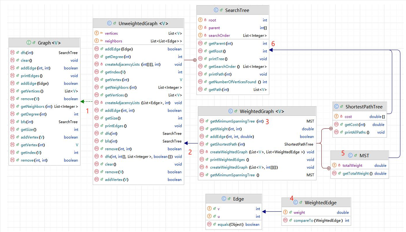
我们需要在UnweightedGraph 类实现这个方法。为此我们需要借助两个类，一个是Edge类，表示图中的边。一个是SeachTree类，可以作为容器存储和打印DFS遍历的结果。
UML如图所示。
在这里插入图片描述
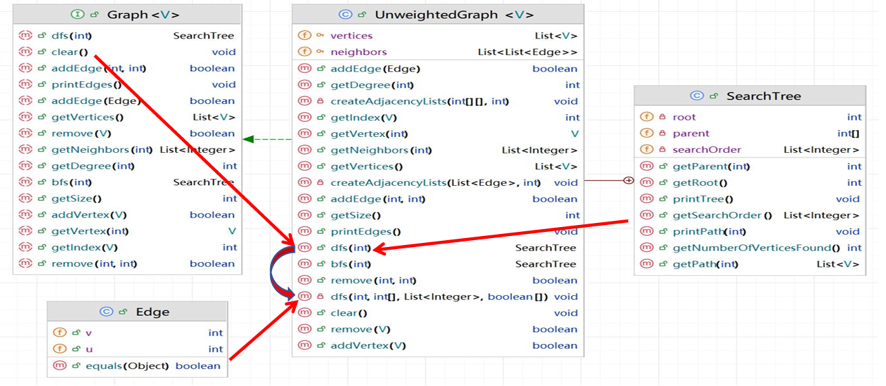
在 UnweightedGraph 类中，私有递归 dfs 方法负责执行实际的DFS操作。
Edge 类表示边，支持DFS操作，通过 $u$ 和 $v$ 属性表示边的起点和终点。
具体代码如下。

public class Edge {
    public int u;
    public int v;

    public Edge(int u, int v) {
        this.u = u;
        this.v = v;
    }

    public boolean equals(Object o) {
        return u == ((Edge) o).u && v == ((Edge) o).v;
    }
}

SearchTree 内部类作为容器，存储和打印DFS遍历的结果。

public class SearchTree {
        private int root; // The root of the tree
        private int[] parent; // Store the parent of each vertex
        private List<Integer> searchOrder; // Store the search order

        /**
         * Construct a tree with root, parent, and searchOrder
         */
        public SearchTree(int root, int[] parent,
                          List<Integer> searchOrder) {
            this.root = root;
            this.parent = parent;
            this.searchOrder = searchOrder;
        }

        /**
         * Return the root of the tree
         */
        public int getRoot() {
            return root;
        }

        /**
         * Return the parent of vertex v
         */
        public int getParent(int v) {
            return parent[v];
        }

        /**
         * Return an array representing search order
         */
        public List<Integer> getSearchOrder() {
            return searchOrder;
        }

        /**
         * Return number of vertices found
         */
        public int getNumberOfVerticesFound() {
            return searchOrder.size();
        }

        /**
         * Return the path of vertices from a vertex to the root
         */
        public List<V> getPath(int index) {
            ArrayList<V> path = new ArrayList<>();

            do {
                path.add(vertices.get(index));
                index = parent[index];
            }
            while (index != -1);

            return path;
        }

        /**
         * Print a path from the root to vertex v
         */
        public void printPath(int index) {
            List<V> path = getPath(index);
            System.out.print("A path from " + vertices.get(root) + " to " +
                    vertices.get(index) + ": ");
            for (int i = path.size() - 1; i >= 0; i--)
                System.out.print(path.get(i) + " ");
        }

        /**
         * Print the whole tree
         */
        public void printTree() {
            System.out.println("Root is: " + vertices.get(root));
            System.out.print("Edges: ");
            for (int i = 0; i < parent.length; i++) {
                if (parent[i] != -1) {
                    // Display an edge
                    System.out.print("(" + vertices.get(parent[i]) + ", " +
                            vertices.get(i) + ") ");
                }
            }
            System.out.println();
        }
    }

SearchTree 类用于存储和打印深度优先搜索（DFS）遍历的结果。
包含三个属性：root（根节点）、parent（每个顶点的父节点数组）和 searchOrder（访问顶点的顺序列表）。
提供了一个构造方法来初始化这些属性，并提供了一个方法来获取树的节点等。

UnweightedGraph 类中的 dfs 方法如下。

// UnweightedGraph 类中的 dfs 方法
public SearchTree dfs(int v) {
    // 一个列表，用于记录访问顶点的顺序
    List<Integer> searchOrder = new ArrayList<>();
    // 一个数组，用于存储DFS树中每个顶点的父节点
    int[] parent = new int[vertices.size()];
    for (int i = 0; i < parent.length; i++)
        parent[i] = -1; // 初始化 parent 数组

    // 一个布尔数组，用于标记顶点是否被访问过
    boolean[] isVisited = new boolean[vertices.size()];
    dfs(v, parent, searchOrder, isVisited);

    // 返回一个新的 SearchTree 对象
    return new SearchTree(v, parent, searchOrder);
}

// 递归的 dfs 方法
private void dfs(int v, int[] parent, List<Integer> searchOrder, boolean[] isVisited) {
    // 标记顶点 v 为已访问
    isVisited[v] = true;
    // 将访问的顶点添加到 searchOrder 列表中
    searchOrder.add(v);

    // 遍历顶点 v 的所有邻居
    for (Edge e : neighbors.get(v)) {
        // 如果邻居 w 未被访问
        if (!isVisited[e.v]) {
            // 将 w 的父节点设置为 v
            parent[e.v] = v;
            // 递归地访问 w
            dfs(e.v, parent, searchOrder, isVisited);
        }
    }
}

dfs(int v) 是一个公共方法，用于从顶点 v 开始执行DFS遍历，并返回一个 SearchTree 对象。
初始化 searchOrder 列表和 parent 数组，并调用私有的递归 dfs 方法。
返回一个新的 SearchTree 对象，包含遍历的结果。
而dfs(int v, int[] parent, List searchOrder, boolean[] isVisited) 是一个私有方法，负责执行实际的递归DFS遍历。
标记当前顶点 v 为已访问，并将其添加到 searchOrder 列表中。
遍历顶点 v 的所有邻居，如果邻居未被访问，则递归地访问该邻居，并更新 parent 数组。

测试代码如下。

public class TestDFS {
  public static void main(String[] args) {
    String[] vertices = {"Seattle", "San Francisco", "Los Angeles",
      "Denver", "Kansas City", "Chicago", "Boston", "New York",
      "Atlanta", "Miami", "Dallas", "Houston"};

    int[][] edges = {
      {0, 1}, {0, 3}, {0, 5},
      {1, 0}, {1, 2}, {1, 3},
      {2, 1}, {2, 3}, {2, 4}, {2, 10},
      {3, 0}, {3, 1}, {3, 2}, {3, 4}, {3, 5},
      {4, 2}, {4, 3}, {4, 5}, {4, 7}, {4, 8}, {4, 10},
      {5, 0}, {5, 3}, {5, 4}, {5, 6}, {5, 7},
      {6, 5}, {6, 7},
      {7, 4}, {7, 5}, {7, 6}, {7, 8},
      {8, 4}, {8, 7}, {8, 9}, {8, 10}, {8, 11},
      {9, 8}, {9, 11},
      {10, 2}, {10, 4}, {10, 8}, {10, 11},
      {11, 8}, {11, 9}, {11, 10}
    };

    Graph<String> graph = new UnweightedGraph<>(vertices, edges);
    UnweightedGraph<String>.SearchTree dfs = 
      graph.dfs(graph.getIndex("Chicago")); 

    java.util.List<Integer> searchOrders = dfs.getSearchOrder();
    System.out.println(dfs.getNumberOfVerticesFound() +
      " vertices are searched in this DFS order:");
    for (int i = 0; i < searchOrders.size(); i++)
      System.out.print(graph.getVertex(searchOrders.get(i)) + " ");
    System.out.println();

    for (int i = 0; i < searchOrders.size(); i++)
      if (dfs.getParent(i) != -1)
        System.out.println("parent of " + graph.getVertex(i) +
          " is " + graph.getVertex(dfs.getParent(i)));
  }
}

DFS的应用如下：

检测图是否连通：通过从任意顶点开始进行DFS遍历，如果遍历的顶点数量与图中顶点的总数相同，则图是连通的；否则，图不是连通的。
查找图中的所有连通分量：对于无向图，DFS可以用来找到所有的连通分量，即图中的每个连通子图。
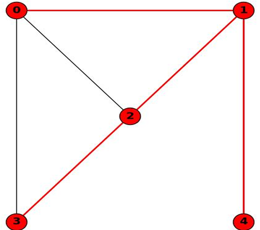
检测两个顶点之间是否存在路径，并找到它（不一定是最短路径）。
如图所示。这里0和2之间的最短路径是0-2，但是DFS的结果是0-1-2。

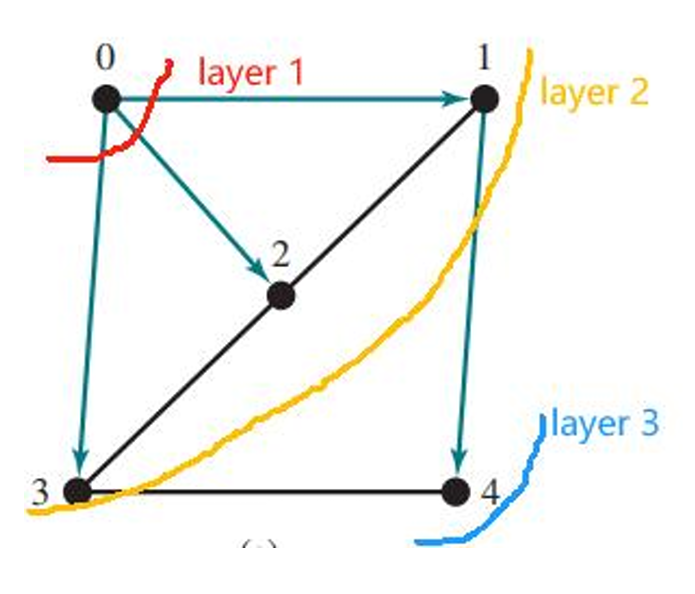
1.3.1.2 广度优先搜索（Breadth-First Search，简称BFS）

广度优先搜索按照从近到远的顺序（即层层向外扩展）访问图中的所有顶点。
在这里插入图片描述
算法的步骤如下：

创建一个空的队列，用于存储待访问的顶点。
将起始顶点 v 加入队列，并标记为已访问。
当队列不为空时，执行以下操作：
从队列中取出（出队）一个顶点，称为 $u$ 。
遍历顶点 $u$ 的所有邻居 $w$ ：
如果邻居 $w$ 未被访问：
将 $w$ 加入队列。
将 $u$ 设置为 $w$ 的父顶点（在BFS树中）。
标记 $w$ 为已访问。

伪代码如下：

bfs(vertex v) {
    // 创建一个空队列用于存储待访问的顶点
    create an empty queue for storing vertices to be visited;
    // 将起始顶点 v 加入队列，并标记为已访问
    add v into the queue;
    mark v visited;
    // 当队列不为空时，执行以下操作
    while the queue is not empty {
        // 从队列中取出一个顶点，称为 u
        dequeue a vertex, say u, from the queue;
        // 遍历顶点 u 的所有邻居 w
        for each neighbor w of u {
            // 如果 w 未被访问
            if w has not been visited {
                // 将 w 加入队列
                add w into the queue;
                // 将 u 设置为 w 的父顶点
                set u as the parent for w;
                // 标记 w 为已访问
                mark w visited;
            }
        }
    }
}

它的时间复杂度为 $O (∣ E ∣ + ∣ V ∣)$ ，与前者一样。
由于每个顶点恰好被访问一次，因此与顶点相关的操作总数是 $∣ V ∣$ 。
由于每条边恰好被访问一次（在检查邻接顶点时），因此与边相关的操作总数是 $∣ E ∣$ 。
因此，算法的总操作数是顶点操作数和边操作数之和，即 $∣ E ∣ + ∣ V ∣$ 。

实现与牵着类似。
在这里插入图片描述
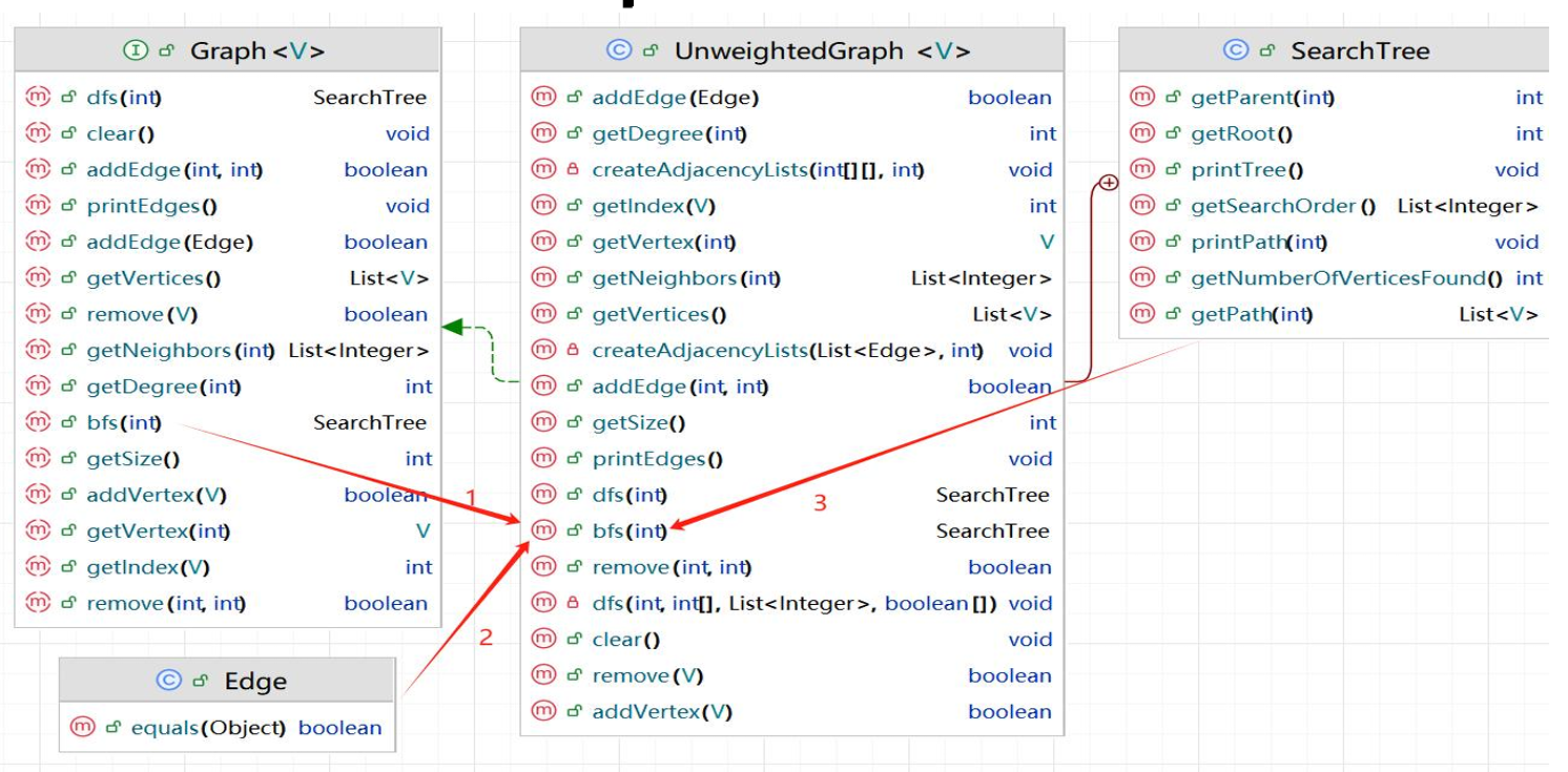
在 UnweightedGraph 类中，私有递归 bfs 方法负责执行实际的BFS操作。用Edge类表示边，支持 BFS 操作。SearchTree 内部类作为容器，存储和打印BFS遍历的结果。
相关的代码如下。

@Override
    /** Starting bfs search from vertex v */
    public SearchTree bfs(int v) {
        List<Integer> searchOrder = new ArrayList<>();
        int[] parent = new int[vertices.size()];
        for (int i = 0; i < parent.length; i++)
            parent[i] = -1; // Initialize parent[i] to -1

        java.util.LinkedList<Integer> queue =
                new java.util.LinkedList<>(); // list used as a queue
        boolean[] isVisited = new boolean[vertices.size()];
        queue.offer(v); // Enqueue v
        isVisited[v] = true; // Mark it visited

        while (!queue.isEmpty()) {
            int u = queue.poll(); // Dequeue to u
            searchOrder.add(u); // u searched
            for (Edge e : neighbors.get(u)) { // Note that e.u is u
                if (!isVisited[e.v]) { // e.v is w in Listing 28.11
                    queue.offer(e.v); // Enqueue w
                    parent[e.v] = u; // The parent of w is u
                    isVisited[e.v] = true; // Mark w visited
                }
            }
        }

        return new SearchTree(v, parent, searchOrder);
    }

测试代码如下。

public class TestBFS {
  public static void main(String[] args) {
    String[] vertices = {"Seattle", "San Francisco", "Los Angeles",
      "Denver", "Kansas City", "Chicago", "Boston", "New York",
      "Atlanta", "Miami", "Dallas", "Houston"};

    int[][] edges = {
      {0, 1}, {0, 3}, {0, 5},
      {1, 0}, {1, 2}, {1, 3},
      {2, 1}, {2, 3}, {2, 4}, {2, 10},
      {3, 0}, {3, 1}, {3, 2}, {3, 4}, {3, 5},
      {4, 2}, {4, 3}, {4, 5}, {4, 7}, {4, 8}, {4, 10},
      {5, 0}, {5, 3}, {5, 4}, {5, 6}, {5, 7},
      {6, 5}, {6, 7},
      {7, 4}, {7, 5}, {7, 6}, {7, 8},
      {8, 4}, {8, 7}, {8, 9}, {8, 10}, {8, 11},
      {9, 8}, {9, 11},
      {10, 2}, {10, 4}, {10, 8}, {10, 11},
      {11, 8}, {11, 9}, {11, 10}
    };

    Graph<String> graph = new UnweightedGraph<>(vertices, edges);
    UnweightedGraph<String>.SearchTree bfs = 
      graph.bfs(graph.getIndex("Chicago")); 

    java.util.List<Integer> searchOrders = bfs.getSearchOrder();
    System.out.println(bfs.getNumberOfVerticesFound() +
      " vertices are searched in this order:");
    for (int i = 0; i < searchOrders.size(); i++)
      System.out.println(graph.getVertex(searchOrders.get(i)));

    for (int i = 0; i < searchOrders.size(); i++)
      if (bfs.getParent(i) != -1)
        System.out.println("parent of " + graph.getVertex(i) + 
          " is " + graph.getVertex(bfs.getParent(i)));
  }
}

BFS的应用有：

检测图是否连通：检测图中任意两个顶点之间是否存在路径，从而判断图是否连通。
也可以通过BFS生成的树（生成树是包含图中所有顶点的无环连通子图）的大小是否与图中顶点的数量相同，可以作为图是否连通的一个指标。
用BFS确定两个特定顶点之间是否存在路径。
查找所有连通分量.
在无权图中找到两个顶点之间的最短路径：因为它是按照边的数量来探索顶点的。即BFS按照离起始顶点的边数来逐层探索顶点，首先探索所有与起始顶点相邻的顶点（1条边），然后是这些顶点的邻居（2条边），以此类推。因此，当BFS第一次到达某个顶点时，它一定是通过最短的可能边数。

1.3.2 有权图

前面我们说的一直是无权图，现在我们说有权图的相关方法如何实现。
首先先有权图是每条边都被赋予了一个权重或者值的图。
在这里插入图片描述
所以现在我们的表示方式也要有所改变。
比如使用边数组（Edge Array）表示加权边的时候，需要加入权重。

int[][] edges = {
    {0, 1, 2}, {0, 3, 8},
    {1, 0, 2}, {1, 2, 7}, {1, 3, 3},
    {2, 1, 7}, {2, 3, 4}, {2, 4, 5},
    {3, 0, 8}, {3, 1, 3}, {3, 2, 4}, {3, 4, 6},
    {4, 2, 5}, {4, 3, 6}
};

同理，使用邻接矩阵（Adjacency Matrix）表示加权边。

Integer[][] adjacencyMatrix = {
    {null, 2, null, 8, null},
    {2, null, 1, 3, null},
    {null, 1, null, 7, 3},
    {null, 3, null, 4, 5},
    {8, 3, 4, null, 6},
    {null, null, 5, 6, null}
};

使用邻接表（Adjacency List）表示加权边。

import java.util.List;
import java.util.ArrayList;

// 一个包含5个列表的数组，每个列表打算存储加权边对象
List<WeightedEdge>[] list = new ArrayList[5];

// 加权边类
public class WeightedEdge implements Comparable<WeightedEdge> {
    // 定义权重
    public double weight;

    // 使用权重构造加权边
    public WeightedEdge(int u, int v, double weight) {
        super(u, v);
        this.weight = weight;
    }

    // 基于权重比较两个边
    public int compareTo(WeightedEdge edge) {
        // 如果当前边的权重大于另一个边，返回1，
        // 如果相等，返回0，
        // 如果小于，返回-1
    }
}

下图展示了现在的UML关系图。
在这里插入图片描述
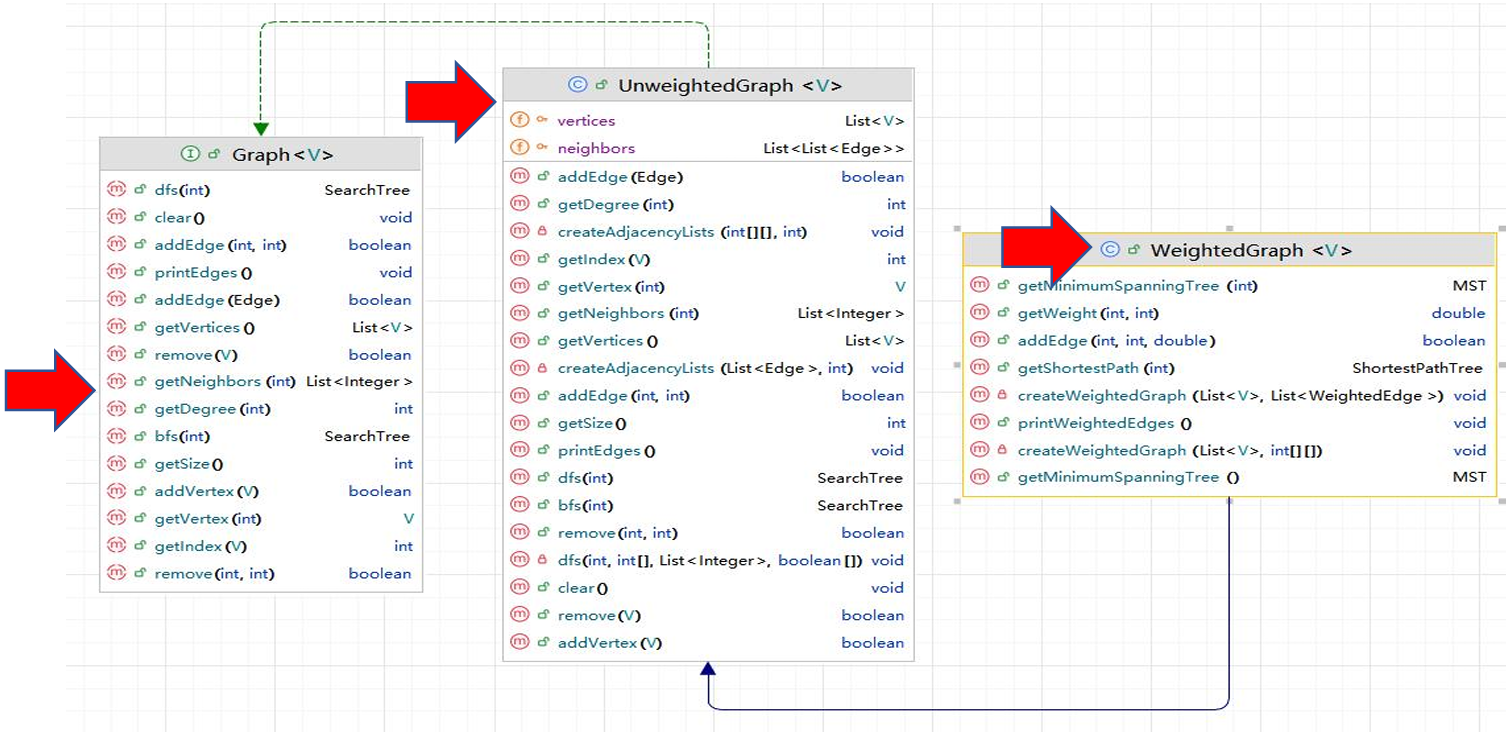
UnweightedGraph类实现了Graph接口，而WeightedGraph类继承自 UnweightedGraph类，添加了处理加权图的额外能力。

1.3.3 最小生成树（Minimum Spanning Tree，简称MST）

在有权图的基础上，我们有最小生成树。
生成树是图 $G$ 的一个连通子图，这个子图是一个树，包含了 $G$ 中所有的顶点。
最小生成树是所有可能的生成树中，边的总权重最小的那一个。
应用如下：

网络设计：在设计网络时，最小生成树可以用来确定连接所有节点的最优方式，以最小化建设成本。
电路设计：在电路设计中，最小生成树可以用来优化电路的布局，减少材料的使用。
数据压缩：在某些数据压缩算法中，最小生成树可以用来减少数据冗余。

我们还需要知道的是一个图可能会有多个最小生成树。

1.3.3.1 Prim算法

算法步骤如下：

初始化：
让 $V$ 表示图中顶点的集合。
让 $T$ 表示生成树中的顶点集合。最初，将起始顶点添加到 $T$ 。
构建生成树：
当 $T$ 的大小小于 $V$ 的大小时（即还有顶点未加入生成树），执行以下操作：
找到 $T$ 中的顶点 $u$ 和 $V - T$ （即不在生成树中的顶点集合）中的顶点 $v$ ，使得边 $(u, v)$ 的权重最小。
将顶点 $v$ 添加到 $T$ 。
伪代码如下。

MST getMinimumSpanningTree(s) {
    Let V denote the set of vertices in the graph;
    Let T be a set for the vertices in the spanning tree;
    Initially, add the starting vertex to T;
    
    while (size of T < n) {
        find u in T and v in V - T with the smallest weight on the edge (u, v), as shown in the figure;
        add v to T;
    }
}

代码如下。

/**
     * Get a minimum spanning tree rooted at vertex 0
     */
    public MST getMinimumSpanningTree() {
        return getMinimumSpanningTree(0);
    }

    /**
     * Get a minimum spanning tree rooted at a specified vertex
     */
    public MST getMinimumSpanningTree(int startingVertex) {
        // cost[v] stores the cost by adding v to the tree
        double[] cost = new double[getSize()];
        for (int i = 0; i < cost.length; i++) {
            cost[i] = Double.POSITIVE_INFINITY; // Initial cost
        }
        cost[startingVertex] = 0; // Cost of source is 0

        int[] parent = new int[getSize()]; // Parent of a vertex
        parent[startingVertex] = -1; // startingVertex is the root
        double totalWeight = 0; // Total weight of the tree thus far

        List<Integer> T = new ArrayList<>();

        // Expand T
        while (T.size() < getSize()) {
            // Find smallest cost u in V - T
            int u = -1; // Vertex to be determined
            double currentMinCost = Double.POSITIVE_INFINITY;
            for (int i = 0; i < getSize(); i++) {
                if (!T.contains(i) && cost[i] < currentMinCost) {
                    currentMinCost = cost[i];
                    u = i;
                }
            }

            if (u == -1) break;
            else T.add(u); // Add a new vertex to T
            totalWeight += cost[u]; // Add cost[u] to the tree

            // Adjust cost[v] for v that is adjacent to u and v in V - T
            for (Edge e : neighbors.get(u)) {
                if (!T.contains(e.v) && cost[e.v] > ((WeightedEdge) e).weight) {
                    cost[e.v] = ((WeightedEdge) e).weight;
                    parent[e.v] = u;
                }
            }
        }

        return new MST(startingVertex, parent, T, totalWeight);
    }

测试代码如下。

public class TestMinimumSpanningTree {
    public static void main(String[] args) {
        String[] vertices = {"Seattle", "San Francisco", "Los Angeles",
                "Denver", "Kansas City", "Chicago", "Boston", "New York",
                "Atlanta", "Miami", "Dallas", "Houston"};

        int[][] edges = {
                {0, 1, 807}, {0, 3, 1331}, {0, 5, 2097},
                {1, 0, 807}, {1, 2, 381}, {1, 3, 1267},
                {2, 1, 381}, {2, 3, 1015}, {2, 4, 1663}, {2, 10, 1435},
                {3, 0, 1331}, {3, 1, 1267}, {3, 2, 1015}, {3, 4, 599},
                {3, 5, 1003},
                {4, 2, 1663}, {4, 3, 599}, {4, 5, 533}, {4, 7, 1260},
                {4, 8, 864}, {4, 10, 496},
                {5, 0, 2097}, {5, 3, 1003}, {5, 4, 533},
                {5, 6, 983}, {5, 7, 787},
                {6, 5, 983}, {6, 7, 214},
                {7, 4, 1260}, {7, 5, 787}, {7, 6, 214}, {7, 8, 888},
                {8, 4, 864}, {8, 7, 888}, {8, 9, 661},
                {8, 10, 781}, {8, 11, 810},
                {9, 8, 661}, {9, 11, 1187},
                {10, 2, 1435}, {10, 4, 496}, {10, 8, 781}, {10, 11, 239},
                {11, 8, 810}, {11, 9, 1187}, {11, 10, 239}
        };

        WeightedGraph<String> graph1 =
                new WeightedGraph<>(vertices, edges);
        WeightedGraph<String>.MST tree1 = graph1.getMinimumSpanningTree();
        System.out.println("Total weight is " + tree1.getTotalWeight());
        tree1.printTree();

        edges = new int[][]{
                {0, 1, 2}, {0, 3, 8},
                {1, 0, 2}, {1, 2, 7}, {1, 3, 3},
                {2, 1, 7}, {2, 3, 4}, {2, 4, 5},
                {3, 0, 8}, {3, 1, 3}, {3, 2, 4}, {3, 4, 6},
                {4, 2, 5}, {4, 3, 6}
        };

        WeightedGraph<Integer> graph2 = new WeightedGraph<>(edges, 5);
        WeightedGraph<Integer>.MST tree2 =
                graph2.getMinimumSpanningTree(1);
        System.out.println("\nTotal weight is " + tree2.getTotalWeight());
        tree2.printTree();
    }
}

现在的UML图如下。
在这里插入图片描述

1.3.3.2 Dijkstra算法

最短路径问题是找到两个顶点之间的最短路径，即总权重（或成本）最小的路径。
算法步骤如下：

初始化：将起始顶点 s 到自身的最短路径距离设为0，到所有其他顶点的最短路径距离设为无穷大。
选择未访问顶点中距离最小的顶点：从起始顶点开始，选择未访问的顶点中，到起始顶点距离最小的顶点。
更新邻居顶点的距离：对于选定顶点的每个邻居顶点，计算从起始顶点经过选定顶点到邻居顶点的距离，如果这个距离小于当前记录的距离，则更新距离。
标记选定顶点为已访问：完成选定顶点的邻居顶点距离更新后，将其标记为已访问。
重复：重复步骤2-4，直到图中所有顶点都被访问。
伪代码如下。

ShortestPathTree getShortestPath(int s) {
    Let T be a set that contains the vertices whose paths to s are known; 
    Set cost[s] = 0; 
    for (each vertex v in V) {
        if (v != s) {
            cost[v] = infinity; 
        }
    }
    
    while (size of T < n) {
        Find u not in T with the smallest cost[u]; 
        Add u to T; 
        for (each edge (u, v) in E) { 
            if (v not in T && cost[v] > cost[u] + w(u, v)) { 
                cost[v] = w(u, v) + cost[u]; 
                parent[v] = u; 
            }
        }
    }
    return new ShortestPathTree();
}

这个算法其实是找到顶点 $s$ 到其他所有顶点的最短路径。

具体代码如下。

/**
     * Find single source shortest paths
     */
    public ShortestPathTree getShortestPath(int sourceVertex) {
        // cost[v] stores the cost of the path from v to the source
        double[] cost = new double[getSize()];
        for (int i = 0; i < cost.length; i++) {
            cost[i] = Double.POSITIVE_INFINITY; // Initial cost set to infinity
        }
        cost[sourceVertex] = 0; // Cost of source is 0

        // parent[v] stores the previous vertex of v in the path
        int[] parent = new int[getSize()];
        parent[sourceVertex] = -1; // The parent of source is set to -1

        // T stores the vertices whose path found so far
        List<Integer> T = new ArrayList<>();

        // Expand T
        while (T.size() < getSize()) {
            // Find smallest cost v in V - T
            int u = -1; // Vertex to be determined
            double currentMinCost = Double.POSITIVE_INFINITY;
            for (int i = 0; i < getSize(); i++) {
                if (!T.contains(i) && cost[i] < currentMinCost) {
                    currentMinCost = cost[i];
                    u = i;
                }
            }

            if (u == -1) break;
            else T.add(u); // Add a new vertex to T

            // Adjust cost[v] for v that is adjacent to u and v in V - T
            for (Edge e : neighbors.get(u)) {
                if (!T.contains(e.v)
                        && cost[e.v] > cost[u] + ((WeightedEdge) e).weight) {
                    cost[e.v] = cost[u] + ((WeightedEdge) e).weight;
                    parent[e.v] = u;
                }
            }
        } // End of while

        // Create a ShortestPathTree
        return new ShortestPathTree(sourceVertex, parent, T, cost);
    }

测试代码如下。

public class TestShortestPath {

    public static void main(String[] args) {

        String[] vertices = {"Seattle", "San Francisco", "Los Angeles",
                "Denver", "Kansas City", "Chicago", "Boston", "New York",
                "Atlanta", "Miami", "Dallas", "Houston"};

        int[][] edges = {
                {0, 1, 807}, {0, 3, 1331}, {0, 5, 2097},
                {1, 0, 807}, {1, 2, 381}, {1, 3, 1267},
                {2, 1, 381}, {2, 3, 1015}, {2, 4, 1663}, {2, 10, 1435},
                {3, 0, 1331}, {3, 1, 1267}, {3, 2, 1015}, {3, 4, 599},
                {3, 5, 1003},
                {4, 2, 1663}, {4, 3, 599}, {4, 5, 533}, {4, 7, 1260},
                {4, 8, 864}, {4, 10, 496},
                {5, 0, 2097}, {5, 3, 1003}, {5, 4, 533},
                {5, 6, 983}, {5, 7, 787},
                {6, 5, 983}, {6, 7, 214},
                {7, 4, 1260}, {7, 5, 787}, {7, 6, 214}, {7, 8, 888},
                {8, 4, 864}, {8, 7, 888}, {8, 9, 661},
                {8, 10, 781}, {8, 11, 810},
                {9, 8, 661}, {9, 11, 1187},
                {10, 2, 1435}, {10, 4, 496}, {10, 8, 781}, {10, 11, 239},
                {11, 8, 810}, {11, 9, 1187}, {11, 10, 239}
        };

        WeightedGraph<String> graph1 =
                new WeightedGraph<>(vertices, edges);
        WeightedGraph<String>.ShortestPathTree tree1 =
                graph1.getShortestPath(graph1.getIndex("Chicago"));
        tree1.printAllPaths();

        // Display shortest paths from Houston to Chicago
        System.out.print("Shortest path from Houston to Chicago: ");
        java.util.List<String> path
                = tree1.getPath(graph1.getIndex("Houston"));
        for (String s : path) {
            System.out.print(s + " ");
        }

        edges = new int[][]{
                {0, 1, 2}, {0, 3, 8},
                {1, 0, 2}, {1, 2, 7}, {1, 3, 3},
                {2, 1, 7}, {2, 3, 4}, {2, 4, 5},
                {3, 0, 8}, {3, 1, 3}, {3, 2, 4}, {3, 4, 6},
                {4, 2, 5}, {4, 3, 6}
        };
        WeightedGraph<Integer> graph2 = new WeightedGraph<>(edges, 5);
        WeightedGraph<Integer>.ShortestPathTree tree2 =
                graph2.getShortestPath(3);
        System.out.println("\n");
        tree2.printAllPaths();
    }
}

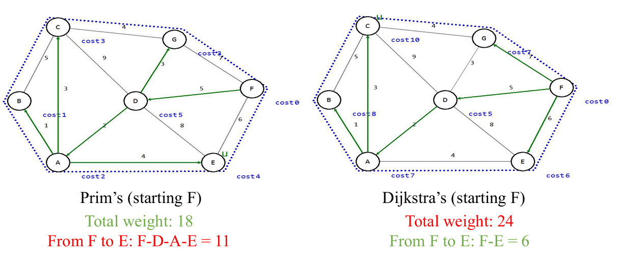
1.3.3.3 Prim算法与Dijkstra算法的对比

Prim算法关注的是如何将新的顶点添加到生成树中，每次迭代都扩展生成树，直到包含所有顶点。
Dijkstra算法关注的是如何从起始顶点到达每个顶点的最短路径，每次迭代都更新到未访问顶点的最短路径。

所以Prim算法的目标是找到最小生成树。
而Dijkstra算法的目标是找到从指定的源顶点 $s$ 到图中所有其他顶点的最短路径。
因此Dijkstra算法的生成树不是最小生成树。
如图所示。
在这里插入图片描述
两者的时间复杂度类似，前面的代码的时间复杂度都是 $O(n^3)$ ，但是经过优化可以到 $O ((E + V) l o g V)$ 。

2.练习

2.1 二分图（Bipartite Graph）

二分图是指图的顶点可以被分成两个互不相交的集合，使得同一集合内的任意两个顶点之间没有边相连。
我们现在使用广度优先搜索（BFS）来判断一个图是否是二分图（Bipartite Graph）。
示例代码如下。

import java.util.*;

public class Graph {
    private int V; // 图的顶点数
    private List<List<Integer>> adj; // 邻接表表示图

    // 构造函数
    public Graph(int V) {
        this.V = V;
        adj = new ArrayList<>();
        for (int i = 0; i < V; i++) {
            adj.add(new ArrayList<>());
        }
    }

    // 添加边
    public void addEdge(int v, int w) {
        adj.get(v).add(w);
        adj.get(w).add(v); // 无向图，添加双向边
    }

    // 判断图是否是二分图
    public boolean isBipartite() {
        // 颜色数组，-1表示未访问，0和1表示两种颜色
        int[] color = new int[V];
        Arrays.fill(color, -1);

        // 遍历所有顶点，处理未访问的顶点
        for (int start = 0; start < V; start++) {
            if (color[start] == -1) { // 如果当前顶点未访问
                if (!bfs(start, color)) {
                    return false; // 如果从某个顶点开始的BFS发现不是二分图，直接返回false
                }
            }
        }
        return true; // 所有连通分量都是二分图
    }

    // BFS辅助方法
    private boolean bfs(int start, int[] color) {
        Queue<Integer> queue = new LinkedList<>();
        queue.add(start);
        color[start] = 0; // 给起始顶点染色为0

        while (!queue.isEmpty()) {
            int u = queue.poll();

            // 遍历u的所有邻接顶点
            for (int v : adj.get(u)) {
                // 如果邻接顶点v未访问，染与u不同的颜色，并加入队列
                if (color[v] == -1) {
                    color[v] = 1 - color[u];
                    queue.add(v);
                } else if (color[v] == color[u]) {
                    // 如果邻接顶点v已访问且与u颜色相同，说明不是二分图
                    return false;
                }
            }
        }
        return true; // BFS完成且未发现冲突
    }

    public static void main(String[] args) {
        Graph g = new Graph(4);
        g.addEdge(0, 1);
        g.addEdge(1, 2);
        g.addEdge(2, 3);
        g.addEdge(3, 0);

        System.out.println("Is the graph bipartite? " + g.isBipartite());
    }
}

2.2 加权图的邻接矩阵表示

示例代码如下。

import java.util.*;

public class WeightedGraph {
    private int V; // 图的顶点数
    private List<List<Edge>> adj; // 邻接表表示图

    // 边的类
    static class Edge {
        int dest; // 目的顶点
        double weight; // 边的权重

        public Edge(int dest, double weight) {
            this.dest = dest;
            this.weight = weight;
        }
    }

    // 构造函数
    public WeightedGraph(int V) {
        this.V = V;
        adj = new ArrayList<>();
        for (int i = 0; i < V; i++) {
            adj.add(new ArrayList<>());
        }
    }

    // 添加边
    public void addEdge(int src, int dest, double weight) {
        adj.get(src).add(new Edge(dest, weight));
        adj.get(dest).add(new Edge(src, weight)); // 无向图，添加双向边
    }

    // 生成邻接矩阵
    public double[][] getAdjacentMatrix() {
        double[][] matrix = new double[V][V];
        for (int i = 0; i < V; i++) {
            for (int j = 0; j < V; j++) {
                matrix[i][j] = Double.POSITIVE_INFINITY; // 初始化为正无穷
            }
        }
        for (int i = 0; i < V; i++) {
            for (Edge edge : adj.get(i)) {
                matrix[i][edge.dest] = edge.weight; // 设置权重
            }
        }
        return matrix;
    }

    public static void main(String[] args) {
        WeightedGraph g = new WeightedGraph(4);
        g.addEdge(0, 1, 1.0);
        g.addEdge(1, 2, 2.0);
        g.addEdge(2, 3, 3.0);
        g.addEdge(3, 0, 4.0);

        double[][] matrix = g.getAdjacentMatrix();
        for (int i = 0; i < 4; i++) {
            for (int j = 0; j < 4; j++) {
                System.out.print(matrix[i][j] + " ");
            }
            System.out.println();
        }
    }
}

2.3 使用邻接矩阵实现Prim算法

与之前使用邻接表的实现不同，这次需要使用邻接矩阵来表示图。
示例代码如下。

import java.util.*;

public class WeightedGraph {
    private int V; // 图的顶点数
    private double[][] adjMatrix; // 邻接矩阵

    // 构造函数
    public WeightedGraph(int V) {
        this.V = V;
        this.adjMatrix = new double[V][V];
        for (int i = 0; i < V; i++) {
            for (int j = 0; j < V; j++) {
                if (i != j) {
                    adjMatrix[i][j] = Double.POSITIVE_INFINITY; // 初始化为正无穷
                }
            }
        }
    }

    // 添加边
    public void addEdge(int src, int dest, double weight) {
        adjMatrix[src][dest] = weight;
        adjMatrix[dest][src] = weight; // 无向图，添加双向边
    }

    // 普里姆算法
    public List<Edge> primMST() {
        boolean[] inMST = new boolean[V]; // 标记顶点是否在MST中
        double[] key = new double[V]; // 最小权重边的权重
        int[] parent = new int[V]; // 父节点数组，用于记录MST的边

        // 初始化
        Arrays.fill(key, Double.POSITIVE_INFINITY);
        key[0] = 0; // 从顶点0开始
        parent[0] = -1; // 顶点0没有父节点

        for (int count = 0; count < V - 1; count++) {
            // 找到不在MST中且key值最小的顶点
            int u = minKey(key, inMST);
            inMST[u] = true; // 将该顶点加入MST

            // 更新相邻顶点的key值
            for (int v = 0; v < V; v++) {
                if (!inMST[v] && adjMatrix[u][v] < Double.POSITIVE_INFINITY &&
                    adjMatrix[u][v] < key[v]) {
                    parent[v] = u;
                    key[v] = adjMatrix[u][v];
                }
            }
        }

        // 构建MST的边列表
        List<Edge> mstEdges = new ArrayList<>();
        for (int i = 1; i < V; i++) {
            mstEdges.add(new Edge(parent[i], i, adjMatrix[parent[i]][i]));
        }
        return mstEdges;
    }

    // 辅助方法：找到不在MST中且key值最小的顶点
    private int minKey(double[] key, boolean[] inMST) {
        double min = Double.POSITIVE_INFINITY;
        int minIndex = -1;
        for (int v = 0; v < V; v++) {
            if (!inMST[v] && key[v] < min) {
                min = key[v];
                minIndex = v;
            }
        }
        return minIndex;
    }

    // 边的类
    public static class Edge {
        int src;
        int dest;
        double weight;

        public Edge(int src, int dest, double weight) {
            this.src = src;
            this.dest = dest;
            this.weight = weight;
        }

        @Override
        public String toString() {
            return "(" + src + " - " + dest + ", weight = " + weight + ")";
        }
    }

    public static void main(String[] args) {
        WeightedGraph g = new WeightedGraph(5);
        g.addEdge(0, 1, 2.0);
        g.addEdge(0, 3, 6.0);
        g.addEdge(1, 2, 3.0);
        g.addEdge(1, 3, 8.0);
        g.addEdge(1, 4, 5.0);
        g.addEdge(2, 4, 7.0);
        g.addEdge(3, 4, 9.0);

        List<Edge> mstEdges = g.primMST();
        System.out.println("Edges in the Minimum Spanning Tree:");
        for (Edge edge : mstEdges) {
            System.out.println(edge);
        }
    }
}