


这一节主要教的是矢量化编程,所以跟机器学习关系其实不大,主要是要对矩阵操作和matlab比较熟悉才行,矢量化编程确实是个很方便的工具,不仅能让代码跑的快,而且代码也会简洁很多很多。
step1:先下好训练用的数据和辅助代码
可以测试下数据和代码,看有没有问题
images = loadMNISTImages('train-images.idx3-ubyte');
labels = loadMNISTLabels('train-labels.idx1-ubyte');

% We are using display_network from the autoencoder code
display_network(images(:,1:100)); % Show the first 100 images
disp(labels(1:10));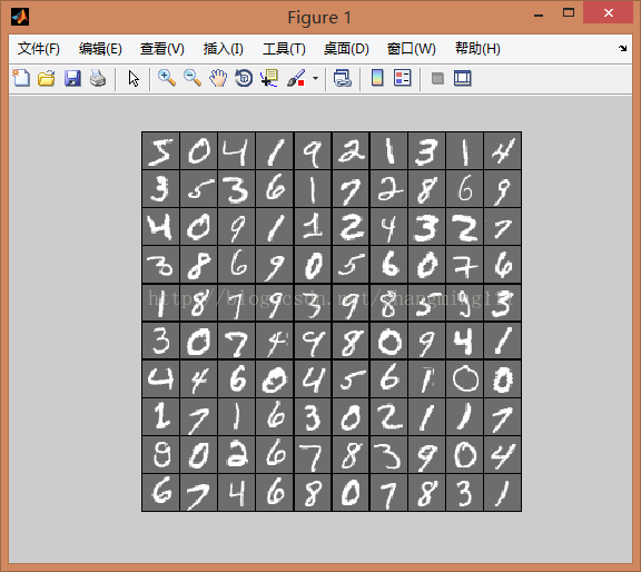
step2:实现sparseAutoencoderCost.m的矢量化和训练
由于我在第一个练习中用的就是适量化了,所以代码不用改,只需要改下训练数据和一些参数的设置,下面还是贴下sparseAutoecoderCost.m的代码
sparseAutoencoderCost.m
function [cost,grad] = sparseAutoencoderCost(theta, visibleSize, hiddenSize, ...
                                             lambda, sparsityParam, beta, data)

% visibleSize: the number of input units (probably 64)
% hiddenSize: the number of hidden units (probably 25)
% lambda: weight decay parameter
% sparsityParam: The desired average activation for the hidden units (denoted in the lecture
%                           notes by the greek alphabet rho, which looks like a lower-case "p").
% beta: weight of sparsity penalty term
% data: Our 64x10000 matrix containing the training data.  So, data(:,i) is the i-th training example.

% The input theta is a vector (because minFunc expects the parameters to be a vector).
% We first convert theta to the (W1, W2, b1, b2) matrix/vector format, so that this
% follows the notation convention of the lecture notes.

W1 = reshape(theta(1:hiddenSize*visibleSize), hiddenSize, visibleSize);
W2 = reshape(theta(hiddenSize*visibleSize+1:2*hiddenSize*visibleSize), visibleSize, hiddenSize);
b1 = theta(2*hiddenSize*visibleSize+1:2*hiddenSize*visibleSize+hiddenSize);
b2 = theta(2*hiddenSize*visibleSize+hiddenSize+1:end);

% Cost and gradient variables (your code needs to compute these values).
% Here, we initialize them to zeros.
cost = 0;
W1grad = zeros(size(W1));
W2grad = zeros(size(W2));
b1grad = zeros(size(b1));
b2grad = zeros(size(b2));

%% ---------- YOUR CODE HERE --------------------------------------
%  Instructions: Compute the cost/optimization objective J_sparse(W,b) for the Sparse Autoencoder,
%                and the corresponding gradients W1grad, W2grad, b1grad, b2grad.
%
% W1grad, W2grad, b1grad and b2grad should be computed using backpropagation.
% Note that W1grad has the same dimensions as W1, b1grad has the same dimensions
% as b1, etc.  Your code should set W1grad to be the partial derivative of J_sparse(W,b) with
% respect to W1.  I.e., W1grad(i,j) should be the partial derivative of J_sparse(W,b)
% with respect to the input parameter W1(i,j).  Thus, W1grad should be equal to the term
% [(1/m) \Delta W^{(1)} + \lambda W^{(1)}] in the last block of pseudo-code in Section 2.2
% of the lecture notes (and similarly for W2grad, b1grad, b2grad).
%
% Stated differently, if we were using batch gradient descent to optimize the parameters,
% the gradient descent update to W1 would be W1 := W1 - alpha * W1grad, and similarly for W2, b1, b2.
%
a1 = sigmoid(bsxfun(@plus,W1 * data,b1)); %hidden层输出
a2 = sigmoid(bsxfun(@plus,W2 * a1,b2)); %输出层输出
p = mean(a1,2); %隐藏神经元的平均活跃度
sparsity = sparsityParam .* log(sparsityParam ./ p) + (1 - sparsityParam) .* log((1 - sparsityParam) ./ (1.-p)); %惩罚因子
cost = sum(sum((a2 - data).^2)) / 2 / size(data,2) + lambda / 2 * (sum(sum(W1.^2)) + sum(sum(W2.^2))) + beta * sum(sparsity); %代价函数
delt2 = (a2 - data) .* a2 .* (1 - a2); %输出层残差
delt1 = (W2' * delt2 + beta .* repmat((-sparsityParam./p + (1-sparsityParam)./(1.-p)),1,size(data,2))) .* a1 .* (1 - a1); %hidden层残差
W2grad = delt2 * a1' ./ size(data,2) + lambda * W2;
W1grad = delt1 * data' ./ size(data,2) + lambda * W1;
b2grad = sum(delt2,2) ./ size(data,2);
b1grad = sum(delt1,2) ./ size(data,2);
%-------------------------------------------------------------------
% After computing the cost and gradient, we will convert the gradients back
% to a vector format (suitable for minFunc).  Specifically, we will unroll
% your gradient matrices into a vector.

grad = [W1grad(:) ; W2grad(:) ; b1grad(:) ; b2grad(:)];

end

%-------------------------------------------------------------------
% Here's an implementation of the sigmoid function, which you may find useful
% in your computation of the costs and the gradients.  This inputs a (row or
% column) vector (say (z1, z2, z3)) and returns (f(z1), f(z2), f(z3)).

function sigm = sigmoid(x)

    sigm = 1 ./ (1 + exp(-x));
end
%% STEP 4: After verifying that your implementation of
%  sparseAutoencoderCost is correct, You can start training your sparse
%  autoencoder with minFunc (L-BFGS).
visibleSize = 28*28;   % number of input units
hiddenSize = 196;     % number of hidden units
sparsityParam = 0.1;   % desired average activation of the hidden units.
                     % (This was denoted by the Greek alphabet rho, which looks like a lower-case "p",
		     %  in the lecture notes).
lambda = 3e-3;     % weight decay parameter
beta = 3;            % weight of sparsity penalty term
theta = initializeParameters(hiddenSize, visibleSize); %  Randomly initialize the parameters
%patches = sampleIMAGES;
images = loadMNISTImages('train-images.idx3-ubyte');
labels = loadMNISTLabels('train-labels.idx1-ubyte');
patches = images(:,1:10000);
%  Use minFunc to minimize the function
addpath minFunc/
options.Method = 'lbfgs'; % Here, we use L-BFGS to optimize our cost
                          % function. Generally, for minFunc to work, you
                          % need a function pointer with two outputs: the
                          % function value and the gradient. In our problem,
                          % sparseAutoencoderCost.m satisfies this.
options.maxIter = 400;	  % Maximum number of iterations of L-BFGS to run
options.display = 'on';


[opttheta, cost] = minFunc( @(p) sparseAutoencoderCost(p, ...
                                   visibleSize, hiddenSize, ...
                                   lambda, sparsityParam, ...
                                   beta, patches), ...
                              theta, options);

%%======================================================================
%% STEP 5: Visualization

W1 = reshape(opttheta(1:hiddenSize*visibleSize), hiddenSize, visibleSize);
display_network(W1', 12);

print -djpeg weights.jpg % save the visualization to a file 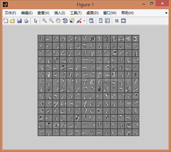


 2195
2195


 被折叠的 条评论
为什么被折叠?
被折叠的 条评论
为什么被折叠?
 到【灌水乐园】发言


