


说明:本文代码为初级练习代码,记录目的主要是为了方便移动端阅读.
一.时间与功率-功率与电流之间的关系import pandas as pd
import numpy as np
from sklearn.model_selection import train_test_split
from sklearn.preprocessing import StandardScaler
from sklearn.linear_model import LinearRegression
# 0.读取数据
path = 'H:/jupyter_notebook/机器学习_线性回归/1、回归、lasso、ridge/datas/household_power_consumption_1000.txt'
# 注意:copy过来的路径是'\',应该改成'/'才正确.
data = pd.read_csv(path,sep=";",low_memory=False)
"""
low_memory:默认为True,在块内部处理文件,导致分析时内存使用量降低,但可能数据类型混乱。要确保没有混合类型设置为False,
或者使用dtype参数指定类型。请注意,不管怎样,整个文件都读入单个DataFrame中,请使用chunksize或iterator参数以块形式返回数据。
(仅在C语法分析器中有效)
"""
# 1.观察数据
print("1.观察数据:\n",data.head(),"\n")
# 2.数据清洗
new_data = data.replace("?",np.NaN)
datas = new_data.dropna(how="any",axis=0)
# 3.提取x,y(涉及到特殊格式字符的处理)
X = datas.iloc[:,0:2]
Y = datas['Global_active_power']
# 将X连接并处理成数字类型
def date_format(dt):
import time
t = time.strptime(' '.join(dt), '%d/%m/%Y %H:%M:%S')
return (t.tm_year, t.tm_mon, t.tm_mday, t.tm_hour, t.tm_min, t.tm_sec)
X = X.apply(lambda x: pd.Series(date_format(x)), axis=1)
print("3.处理后的X:\n",X.head(),"\n")
# 4.划分训练集测试集
X_train,X_test,Y_train,Y_test = train_test_split(X,Y,train_size=0.8,random_state=0)
'''
from sklearn.model_selection import train_test_split
train_test_split:
参数:
*arrays: Allowed inputs are lists, numpy arrays, scipy-sparse matrices or pandas dataframes.
test_size: By default, the value is set to 0.25. The default will change in version 0.21.
train_size: If None, the value is automatically set to the complement(互补) of the test size.
random_state: default=None
shuffle(洗牌): boolean, optional (default=True),If shuffle=False then stratify must be None.
stratify: array-like or None (default is None),If not None, data is split in a stratified fashion,
using this as the class labels.
'''
# 5.数据标准化
ss = StandardScaler()
X_train = ss.fit_transform(X_train) # 训练并转换
X_test = ss.transform(X_test) #直接使用前面的转换规则
'''
from sklearn.preprocessing import StandardScaler
Parameters:
copy : boolean, optional, default True
If False, try to avoid a copy and do inplace scaling instead. This is not guaranteed to always work inplace;
e.g. if the data is not a NumPy array or scipy.sparse CSR matrix, a copy may still be returned.
with_mean : boolean, True by default
If True, center the data before scaling. This does not work (and will raise an exception) when attempted on
sparse matrices, because centering them entails building a dense matrix which in common use cases is likely
to be too large to fit in memory.
with_std : boolean, True by default
If True, scale the data to unit variance (or equivalently, unit standard deviation).
Methods:
fit(X[, y]) --- Compute the mean and std to be used for later scaling.
fit_transform(X[, y]) --- Fit to data, then transform it.
get_params([deep]) --- Get parameters for this estimator.
inverse_transform(X[, copy]) --- Scale back the data to the original representation
partial_fit(X[, y]) --- Online computation of mean and std on X for later scaling.
set_params(**params) --- Set the parameters of this estimator.
transform(X[, y, copy]) --- Perform standardization by centering and scaling
'''
# 6.建立模型
lr = LinearRegression()
lr.fit(X_train,Y_train)
'''
from sklearn.linear_model import LinearRegression
Methods:
fit(X, y[, sample_weight]) --- Fit linear model.
get_params([deep]) --- Get parameters for this estimator.
predict(X) --- Predict using the linear model
score(X, y[, sample_weight]) --- Returns the coefficient of determination R^2 of the prediction.
set_params(**params) --- Set the parameters of this estimator.
Attributes:
coef_ :特征系数
intercept_:截距项
'''
y_predict = lr.predict(X_test)
print("准确率:",lr.score(X_train,Y_train))
print("mse:",np.average((y_predict-Y_test)**2))
print("rmse:",np.sqrt(np.average((y_predict-Y_test)**2)))
print("特征系数:",lr.coef_)
print("截距项:",lr.fit_intercept)
# 7.保存模型
from sklearn.externals import joblib
joblib.dump(ss,"data_ss.model")
joblib.dump(lr,"data_lr.model")
joblib.load("data_ss.model")
joblib.load("data_lr.model")
# 8.作图
from matplotlib import pyplot as plt
import matplotlib as mpl
## 设置字符集,防止中文乱码
mpl.rcParams['font.sans-serif']=[u'simHei']
mpl.rcParams['axes.unicode_minus']=False
plt.figure()
t = np.arange(len(X_test))
y1 = Y_test
y2 = y_predict
plt.plot(t,y1,'r-',label="真实值",linewidth=2)
plt.plot(t,y2,'g-',label="预测值",linewidth=2)
plt.legend()
plt.title("时间与功率的关系")
plt.grid()
plt.show()
# 功率与电流的关系
X2 = datas.iloc[:,2:4]
Y2 =datas.iloc[:,5]
X2_train,X2_test,Y2_train,Y2_test = train_test_split(X2,Y2,train_size=0.8,random_state=0)
ss2 = StandardScaler()
X2_train = ss2.fit_transform(X2_train)
X2_test = ss2.transform(X2_test)
lr2 = LinearRegression()
lr2.fit(X2_train,Y2_train)
y2_predict = lr2.predict(X2_test)
print("y2预测值:",y2_predict)
print("准确率:",lr2.score(X2_train,Y2_train))
print("mse:",np.average((y2_predict-Y2_test)**2))
print("相关系数",lr2.coef_)
plt.figure()
x2 = np.arange(len(X_test))
y21 = Y2_test
y22 = y2_predict
plt.plot(x2,y21,'r-',linewidth=2,label="y2真实值")
plt.plot(x2,y22,'g-',linewidth=2,label="y2预测值")
plt.legend()
plt.grid()
plt.show()
1.观察数据:
          Date      Time  Global_active_power  Global_reactive_power  Voltage  \
0  16/12/2006  17:24:00                4.216                  0.418   234.84
1  16/12/2006  17:25:00                5.360                  0.436   233.63
2  16/12/2006  17:26:00                5.374                  0.498   233.29
3  16/12/2006  17:27:00                5.388                  0.502   233.74
4  16/12/2006  17:28:00                3.666                  0.528   235.68

   Global_intensity  Sub_metering_1  Sub_metering_2  Sub_metering_3
0              18.4             0.0             1.0            17.0
1              23.0             0.0             1.0            16.0
2              23.0             0.0             2.0            17.0
3              23.0             0.0             1.0            17.0
4              15.8             0.0             1.0            17.0

3.处理后的X:
       0   1   2   3   4  5
0  2006  12  16  17  24  0
1  2006  12  16  17  25  0
2  2006  12  16  17  26  0
3  2006  12  16  17  27  0
4  2006  12  16  17  28  0

准确率: 0.24409311805909026
mse: 1.355110989954378
rmse: 1.164092345973625
特征系数: [ 0.00000000e+00  1.11022302e-16 -1.41588166e+00 -9.34953243e-01
 -1.02140756e-01  0.00000000e+00]
截距项: True
y2预测值: [ 9.7986423   1.81470527  3.62631391  1.22006358  5.83536396  5.66629897
 13.60417919 14.41065542 10.21254934 14.45499821 13.64366735  1.24470041
  4.15025609 11.97982693  3.03187754 12.06027088  8.21375473 13.95730716
 17.34265582  9.71487589 15.84289083 18.82718817 10.02529883  8.26130264
  9.86597829  5.53486732 18.79113393 15.28447351  6.01615141 22.71677893
  1.81798079 14.70794107 10.31932069  2.8855887  11.0963172   1.84419672
  7.05078114 10.73488895 10.03183815 14.83612066 14.21188778  9.80521095
 10.36201984 14.36466901  8.03625453  6.26081746  1.2857618  14.23004397
  9.87091504  9.93824516 10.64292786  9.99898904 13.76190304  2.02821277
 10.27332841  8.74592092 12.51040815 14.75235425  9.8856901   9.95960647
  9.92507853  2.20075861 14.23825625 14.82460939  3.73969497 13.68470528
 14.79505927  9.60158869 13.53848097 10.96323605  9.88240284 10.36693899
  3.86441718  8.34832111  9.747725    2.23356666  8.5536574   3.31098941
  3.71659617  4.14203794  8.04122062  4.48855032 16.25518944  6.36916205
  9.99409922 14.45007319 14.41229905 11.41979531 18.82718817  9.747725
  4.30955903 15.54397916  1.26112497 14.22010006  3.16971945  8.89033147
  1.19542674 14.44183158 10.83345976 10.51813526 13.50401756  9.75265002
 12.33948834 10.73164863  2.13983874 10.27496617  3.5294102   5.04376839
 10.24535738 13.88672498 15.25489992  2.40600104 20.46811752  2.94471241
 13.96720413  5.30156587 10.41129938 11.29820783  9.42748721 11.21287405
 11.02722025  2.20239637 15.28774903 18.78453594 14.52395436 10.04007976
 10.72341288  7.02289225 29.45723389 10.5147776   7.31365031 10.3784444
  9.9743522   1.86235291  2.25002641 10.21911212  1.92631951 15.83000579
  9.00864342  9.75758091 14.39424847  9.79866577 10.3784444  14.17903867
 13.41529679 10.11892115 10.76933476 11.02556488 18.71221627 17.17663757
  9.97774506 11.51826051 10.67087542  2.19582186 10.65278964  1.45000737
  2.11520191 10.19608371  7.54850152 16.52775025 11.80585452  9.89554601
 14.71288369 10.22241111  9.81834825 10.12877706  9.9513942  25.19170382
  1.93453179  1.48285648 18.92414467  3.29784037 14.45835     1.79006257
 15.8182716  10.99114254 14.3958745   2.21061452  2.9479762  14.3565154
 10.18955613 12.93901985 15.893902    9.86927141  2.17268785  1.45000737
 10.4030871  11.40991007 10.3784444  14.59630923  9.89222942 10.11072061
 10.48684178 15.23215898  1.79170033 14.18401649 10.53284579 13.99348459
  2.1038549  13.61079477]
准确率: 0.9909657573073489
mse: 0.20934469544344503
相关系数 [5.07744316 0.07191391]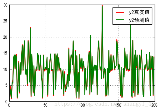
二.时间与电压的多项式关系import pandas as pd
import numpy as np
from matplotlib import pyplot as plt
import matplotlib as mpl
from sklearn.model_selection import train_test_split
from sklearn.preprocessing import StandardScaler
from sklearn.linear_model import LinearRegression
mpl.rcParams['font.sans-serif']=[u'simHei']
mpl.rcParams['axes.unicode_minus']=False
path = 'H:/jupyter_notebook/机器学习_线性回归/1、回归、lasso、ridge/datas/household_power_consumption_1000.txt'
data = pd.read_csv(path,sep=";",low_memory=False)
print(data.head())
data1 = data.replace("?",np.NaN)
data2 = data.dropna(axis=0,how="any")
x = data2.iloc[:,0:2]
y = data2["Voltage"]
def format_time(dt):
import time
t = time.strptime(" ".join(dt),"%d/%m/%Y %H:%M:%S")
return (t.tm_year, t.tm_mon, t.tm_mday, t.tm_hour, t.tm_min, t.tm_sec)
x_new = x.apply(lambda x:pd.Series(format_time(x)),axis=1)
print(x_new.head(),"\n")
x = x_new
x_train,x_test,y_train,y_test = train_test_split(x,y,train_size=0.8,random_state=123)
ss = StandardScaler()
x_train = ss.fit_transform(x_train)
x_test = ss.transform(x_test)
lr = LinearRegression()
lr.fit(x_train,y_train)
y_predict = lr.predict(x_test)
print("y的预测值:",y_predict,"\n")
print("score:",lr.score(x_test,y_test))
print("mse:",np.average((y_predict-y_test)**2))
print("特征系数:",lr.coef_)
print("截距项:",lr.intercept_)
plt.figure()
x = np.arange(len(x_test))
plt.plot(x,y_test,"r-",label="真实值")
plt.plot(x,y_predict,"b-",label="预测值")
plt.legend()
plt.show()输出:
   Date      Time  Global_active_power  Global_reactive_power  Voltage  \
0  16/12/2006  17:24:00                4.216                  0.418   234.84
1  16/12/2006  17:25:00                5.360                  0.436   233.63
2  16/12/2006  17:26:00                5.374                  0.498   233.29
3  16/12/2006  17:27:00                5.388                  0.502   233.74
4  16/12/2006  17:28:00                3.666                  0.528   235.68

   Global_intensity  Sub_metering_1  Sub_metering_2  Sub_metering_3
0              18.4             0.0             1.0            17.0
1              23.0             0.0             1.0            16.0
2              23.0             0.0             2.0            17.0
3              23.0             0.0             1.0            17.0
4              15.8             0.0             1.0            17.0
      0   1   2   3   4  5
0  2006  12  16  17  24  0
1  2006  12  16  17  25  0
2  2006  12  16  17  26  0
3  2006  12  16  17  27  0
4  2006  12  16  17  28  0

y的预测值: [236.05032034 236.21867561 235.81862036 242.24894689 236.09958844
 242.57974703 236.42165844 242.05300237 242.94291894 242.17969178
 236.1623692  236.00696264 236.26090541 236.43517109 235.88787548
 236.41462014 242.47248068 236.36535203 236.37999258 242.08171952
 236.39294129 236.21754772 236.06326905 242.74584651 242.3122916
 243.0197763  242.63492554 236.06496089 242.6473103  235.85437581
 242.53638933 235.76935226 242.45362156 236.34423713 242.92940628
 242.68419365 236.25921357 236.14885655 236.20994547 242.2841384
 242.54286369 236.13956246 242.58678533 236.29496903 242.67068099
 242.65660439 236.15363906 242.78103802 236.35127543 236.25217527
 235.92306698 242.28470234 242.6484382  242.89365083 236.4985158
 236.1694075  242.35395746 235.96529678 242.3334065  236.5337073
 242.76808931 242.24247254 236.00048829 242.61972105 236.07087129
 242.39562332 242.6343616  242.44601931 242.89308688 235.99344999
 236.20290717 242.56341464 242.6121188  236.16293315 242.32693215
 242.31172765 242.93531669 243.01330194 236.0849479  242.40378951
 242.22248553 236.32368617 242.80328081 242.29286854 242.47304462
 235.93066923 242.41026386 243.0338529  242.14506422 235.84029921
 242.29765105 243.0408912  242.99922534 235.75527565 236.07143524
 242.70305276 242.84551062 243.0971976  242.78216591 242.39731516
 242.93644458 243.00626364 242.83790837 242.88717648 242.690668
 242.97107214 236.18292016 242.49359558 242.71009106 235.80454376
 242.60564445 242.46713422 236.33719883 242.28583024 236.31608393
 242.07468121 242.48881307 242.92180403 235.85324792 242.27766404
 242.71065501 242.43841707 236.05144823 242.89421478 242.88661253
 235.84620962 242.6836297  235.83269696 236.19756071 235.83326091
 242.80862727 242.33509834 242.48008293 242.15857688 242.11634707
 242.3474831  242.33988086 236.10549885 242.6977063  242.94235499
 236.21050942 242.80271687 236.28849467 235.86788847 235.94418188
 242.45136578 242.35339351 235.85381186 242.90012518 236.00218013
 242.93588063 236.1131011  242.50176177 242.63548949 236.41405619
 242.73289781 236.28089242 235.84677356 235.95178413 242.66364269
 236.22571391 242.75992312 236.24570092 236.28145637 236.02329503
 242.22192158 242.82383177 235.72008415 235.93010528 242.20080668
 242.79624251 242.72529556 242.65491255 242.92884233 242.69123195
 236.4774009  242.72642345 235.83213302 242.64252779 236.04215414
 242.01781086 241.9409535  242.53695328 236.33072448 236.39997959
 242.55806818 242.99218704 236.0919862  236.47092654 242.82439572
 236.5055541  236.01569278 242.52878708 242.74050005 236.19586887
 236.02273108 236.03567979 242.41730217 236.26794371 236.456286  ]

score: 0.531897455363159
mse: 7.5041855671999995
特征系数: [0.00000000e+00 2.22044605e-16 3.76295063e+00 6.78297825e-01
 1.20843263e-01 0.00000000e+00]
截距项: 240.028425
# 多项式
from sklearn.pipeline import Pipeline
from sklearn.preprocessing import PolynomialFeatures

model = Pipeline([
        ("Poly",PolynomialFeatures()),
        ("Linear",LinearRegression())
    ])

x2 = data2.iloc[:,0:2]
y2 = data2["Voltage"]

def format_time(dt):
    import time
    t = time.strptime(" ".join(dt),"%d/%m/%Y %H:%M:%S")
    return (t.tm_year, t.tm_mon, t.tm_mday, t.tm_hour, t.tm_min, t.tm_sec)

x2_new = x2.apply(lambda x2:pd.Series(format_time(x2)),axis=1)
x2 = x2_new

x2_train,x2_test,y2_train,y2_test = train_test_split(x2,y2,train_size=0.8,random_state=123)

ss = StandardScaler()
x2_train = ss.fit_transform(x2_train)
x2_test = ss.transform(x2_test)

d = 9
model.set_params(Poly__degree=d)
lin = model.get_params()["Linear"]
model.fit(x2_train,y2_train)

y2_predict = model.predict(x2_test)
print("得分:",model.score(x2_train,y2_train))

x = np.arange(len(x2_test))
plt.plot(x,y2_test,"r-",label="真实值",linewidth=2)
plt.plot(x,y2_predict,"b-",label="预测值",linewidth=2)
plt.legend()
plt.show()
输出:
得分: 0.9290211106400875
# 综合绘图
N = 10
d_pool = np.arange(1,N,1)
m = d_pool.size


clrs = []
for c in np.linspace(16711680,255,m):
    clrs.append("#%06x"%int(c))

plt.figure(figsize=(20,18),facecolor="w")
score_list = []
for i,d in enumerate(d_pool):
    plt.subplot(N-1,1,i+1) # 控制画图位置,n-1代表行位,1代表列位,i+1代表位置
    plt.plot(x,y2_test,"r-",label="真实值",zorder=N)
    model.set_params(Poly__degree=d)
    lin = model.get_params()["Linear"]
    model.fit(x2_train,y2_train)
    s = model.score(x2_train,y2_train)
    score_list.append(s)
    print("{0}阶,准确率为:{1}".format(d,s))
    label2 = "{}阶,准确率为:{:.3%}".format(d,s)
    plt.plot(x,y2_predict,color=clrs[i],lw=3,alpha=0.75,label=label2)
    plt.legend(loc="upper left")
    plt.grid()
    plt.ylabel("{}阶结果".format(d))

plt.suptitle("线性回归预测时间与功率之间的多项式关系",fontsize=20)
plt.grid()
plt.show()
输出:
1阶,准确率为:0.5792954707774683
2阶,准确率为:0.7670483283461779
3阶,准确率为:0.8427881170421129
4阶,准确率为:0.8484100419413363
5阶,准确率为:0.8588631436136849
6阶,准确率为:0.89065925236302
7阶,准确率为:0.9081147920237467
8阶,准确率为:0.9244417146081483
9阶,准确率为:0.9290211106400875
三.过拟合样例代码及集中算法的多项式过拟合比较import numpy as np
import pandas as pd
from matplotlib import pyplot as plt
import matplotlib as mpl
from sklearn.pipeline import Pipeline
from sklearn.preprocessing import PolynomialFeatures
from sklearn.linear_model import LinearRegression,RidgeCV,LassoCV,ElasticNetCV
mpl.rcParams['font.sans-serif']=[u'simHei']
mpl.rcParams['axes.unicode_minus']=False
# 创建模拟数据
np.random.seed(123)
np.set_printoptions(linewidth=1000,suppress=True) # 显示方式设置
N = 10
x = np.linspace(0,6,N) + np.random.randn(N)
y = 1.8*x**3 + x**2 - 14*x - 7 + np.random.randn(N)
x.shape = -1,1
y.shape = -1,1
# print(x,x.shape,"\n")
# print(y,y.shape,"\n")
models = [
Pipeline([
("Poly",PolynomialFeatures()),
("Linear",LinearRegression())
]),
Pipeline([
("Poly",PolynomialFeatures()),
("Linear",RidgeCV(alphas=np.logspace(-3,2,50)))
]),
Pipeline([
("Poly",PolynomialFeatures()),
("Linear",LassoCV(alphas=np.logspace(-3,2,50)))
]),
Pipeline([
("Poly",PolynomialFeatures()),
("Linear",ElasticNetCV(alphas=np.logspace(-3,2,50),l1_ratio=[0.1,0.5,0.7,0.9,0.95,1]))
])
]
# 线性模型过拟合图形识别
plt.figure(facecolor="w",figsize=(15,10))
degree = np.arange(1,N,2) # 跳2阶显示 : [1,3,5,7,9]
dm = degree.size # 前面N=10,故这里dm=3
color = []
for c in np.linspace(16711680,255,dm):
color.append("#%06x"%int(c))
model = models[0]
for i,d in enumerate(degree):
plt.subplot(int(np.ceil(dm/2.0)),2,i+1) # np.ceil() :向正无穷取整 朝正无穷大方向取整
plt.plot(x,y,"ro",ms=10,zorder=N) # ms设置o的大小
model.set_params(Poly__degree=d)
model.fit(x,y)
'''
alpha : 透明度,值在0到1之间,0为完全透明,1为完全不透明
animated : 布尔值,在绘制动画效果时使用
axes : 此Artist对象所在的Axes对象,可能为None
clip_box : 对象的裁剪框
clip_on : 是否裁剪
clip_path : 裁剪的路径
contains : 判断指定点是否在对象上的函数
figure : 所在的Figure对象,可能为None
label : 文本标签
picker : 控制Artist对象选取
transform : 控制偏移旋转
visible : 是否可见
zorder : 控制绘图顺序
'''
lin = model.get_params()["Linear"]
print("{}阶,系数为{}".format(d,lin.coef_.ravel()))
x_hat = np.linspace(x.min(),x.max(),num=100) # 产生模拟数据
x_hat.shape = -1,1
y_hat = model.predict(x_hat)
s = model.score(x,y)
z = N -1 if (d == 2) else 0
label = "{}阶,正确率为{:.3%}".format(d,s)
plt.plot(x_hat,y_hat,color=color[i],lw=2,alpha=0.75,label = label,zorder=z) # lw=linewidth ls=linestyle
plt.legend(loc="upper left")
plt.grid()
plt.xlabel("X",fontsize=16)
plt.ylabel("Y",fontsize=16)
plt.tight_layout(1,rect=(0,0,1,0.95)) # 图像外部边缘的调整可以使用plt.tight_layout()进行自动控制,此方法不能够很好的控制图像间的间隔
plt.suptitle("线性回归过拟合显示",fontsize=16)
plt.show()输出:
1阶,系数为[ 0.         54.99809434]
3阶,系数为[  0.         -13.37052062   0.84335416   1.81181463]
5阶,系数为[  0.         -13.95366847   1.11179761   2.07426776  -0.1061305    0.0094719 ]
7阶,系数为[  0.          26.99888892  -8.82195648 -23.87928912  20.4292752   -6.09809543   0.81494919  -0.04069   ]
9阶,系数为[    0.         -7371.75279564  7199.48273329   845.0961721  -5826.32754044  4231.55142855 -1465.01578073   272.83020628   -26.26814082     1.0261812 ]
# 线性回归.Ridge回归.Lasso回归.Elastic Net比较
# 线性模型过拟合图形识别
plt.figure(facecolor="w",figsize=(20,18))
degree = np.arange(1,N,2)
dm = degree.size  # 前面N=10,故这里dm=3

color = []
for c in np.linspace(16711680,255,dm):
    color.append("#%06x"%int(c))

for t in range(len(models)):
    model = models[t]
    plt.subplot(2,2,t+1)
    plt.plot(x,y,"ro",ms=10,zorder=N)  # ms设置o的大小

    for i,d in enumerate(degree):
        model.set_params(Poly__degree=d)
        model.fit(x,y)

        lin = model.get_params()["Linear"]
        print("{}阶,系数为{}".format(d,lin.coef_.ravel()))

        x_hat = np.linspace(x.min(),x.max(),num=100) # 产生模拟数据
        x_hat.shape = -1,1
        y_hat = model.predict(x_hat)
        s = model.score(x,y)

        label = "{}阶,正确率为{:.3%}".format(d,s)
        plt.plot(x_hat,y_hat,color=color[i],lw=2,alpha=0.75,label = label) # lw=linewidth ls=linestyle

        plt.legend(loc="upper left")
        plt.grid()
        plt.xlabel("X",fontsize=16)
        plt.ylabel("Y",fontsize=16)

plt.tight_layout(1,rect=(0,0,1,0.95))  # 图像外部边缘的调整可以使用plt.tight_layout()进行自动控制,此方法不能够很好的控制图像间的间隔
plt.suptitle("线性回归过拟合显示",fontsize=16)
plt.show()
输出:
(系数输出内容略去,仅观察图)


 2021
2021

 被折叠的 条评论
为什么被折叠?
被折叠的 条评论
为什么被折叠?
 到【灌水乐园】发言


