Human-Like Machine Hearing With AI (2/3)--The importance of memory

文章来自

Author ：Daniel Rothmann

原文网站：链接

未翻译...

Hi, and welcome back! This article series details a framework for real-time audio signal processing with AI which I have worked on in cooperation with Aarhus University and intelligent loudspeaker manufacturer Dynaudio.

If you’ve missed out on the previous articles, click below to get up to speed:

Background: The promise of AI in audio processing
Criticism: What’s wrong with CNNs and spectrograms for audio processing?
Part 1: Human-Like Machine Hearing With AI (1/3)

In the previous part, we mapped the fundamentals of how humans experience sound as spectral impressions formed in the cochlea which are then “coded” by a sequence of brainstem nuclei. This article will explore how we can integrate memory when producing spectral sounds embeddings with an artificial neural network for sound understanding.

Echoic memory

The meaning of a sound event arises, in large part, from the temporal interplay between spectral features.

One demonstration of this can be seen in the fact that the human auditory system encodes identical phonemes of speech in different ways depending on their temporal context [1]. That means that a phoneme /e/ can mean different things to us neurologically, depending on what came before it.

Memory is crucial to performing sound analysis since it is only possible to compare impressions of “the moment” to previous impressions if they are actually stored somewhere.

Human short term memory is made up of an collection of components which integrate both sensory and working memory [2]. In examination of sound perception, auditory sensory memory (sometimes referred to as echoic memory) has been found in humans. C. Alain et. al. describe auditory sensory memory as “a critical first stage in auditory perception that permits listeners to integrate incoming acoustic information with stored representations of preceding auditory events” [2].

Computationally, we can think of echoic memory as a short buffer of immediate auditory impressions.

There has been disagreements about the duration of echoic memory. On the basis of pure-tone and spoken-vowel masking studies, D. Massaro has argued for ~250 ms while A. Treisman argued for ~4 seconds based on a dichotic listening experiment [3]. For the purpose of integrating the idea of echoic memory with neural networks, we might not need to settle on a fixed duration of sensory store but we can experiment with memory within a range of a few seconds.

Going in circles

Implementing sensory memory in digital spectral representations could be quite straightforward. We can simply allocate a circular buffer to store a predetermined number of spectra at previous timesteps.

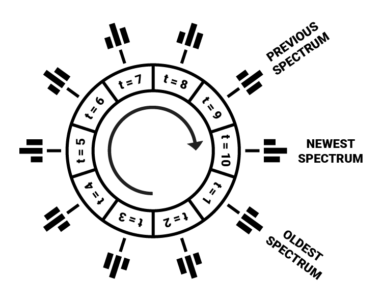
                      An illustrated circular buffer for holding spectral memory (where t denotes the timestep).

A circular buffer is a data structure consisting of an array which is treated as circular, where its indices loop back to 0 after the array’s length is reached [4].

In our case, this could be a multidimensional array with the length of the desired amount of memory, each indice of the circular buffer holding a full frequency spectrum for a specific timestep. As new spectra are calculated, they are written to the buffer, overwriting the oldest timesteps if the buffer is already full.

As the buffer fills, two pointers are updated: A tail pointer marking the newest element added and a head pointer marking the oldest element and, as such, the beginning of the buffer [4].

Here is an example of a circular buffer in Python adapted from Eric Wieser:

import numpy as np
class CircularBuffer():
    # Initializes NumPy array and head/tail pointers
    def __init__(self, capacity, dtype=float):
        self._buffer = np.zeros(capacity, dtype)
        self._head_index = 0
        self._tail_index = 0
        self._capacity = capacity
    # Makes sure that head and tail pointers cycle back around
    def fix_indices(self):
        if self._head_index >= self._capacity:
            self._head_index -= self._capacity
            self._tail_index -= self._capacity
        elif self._head_index < 0:
            self._head_index += self._capacity
            self._tail_index += self._capacity
    # Inserts a new value in buffer, overwriting old value if full
    def insert(self, value):
        if self.is_full():
            self._head_index += 1
        self._buffer[self._tail_index % self._capacity] = value
        self._tail_index += 1
        self.fix_indices()
        
    # Returns the circular buffer as an array starting at head index
    def unwrap(self):
        return np.concatenate((
            self._buffer[self._head_index:min(self._tail_index, self._capacity)],
            self._buffer[:max(self._tail_index - self._capacity, 0)]
        ))
    # Indicates whether the buffer has been filled yet
    def is_full(self):
        return self.count() == self._capacity
    # Returns the amount of values currently in buffer
    def count(self):
        return self._tail_index - self._head_index

Reducing input size

In order to store a full second of frequency spectra at a resolution of 5 ms per timestep, a buffer with a capacity of 200 elements are needed. Each of these elements would contain an array of frequency magnitudes. If human-like spectral resolution is desired, those arrays would contain 3500 values. For a total of 200 timesteps, that is 700,000 values to be processed.

If passed to an artificial neural network, an input with a length of 700,000 values runs the risk of being computationally expensive. This risk can be mitigated by reducing the spectral and temporal resolution or keeping a shorter duration of spectral information in memory.

We can also draw inspiration from the Wavenet architecture, which utilizes dilated causal convolutions in order to optimize analysis of the large amount of sequential data in raw sample audio. As explained by A. Van Den Oord et al.,“A dilated convolution (also called á trous, or convolution with holes) is a convolution where the filter is applied over an area larger than its length by skipping input values with a certain step” [5].

Under the assumption that the most recent incoming frequency data is the largest determining factor in momentary sound analysis, a dilated spectral buffer could be a useful tool for reducing the size of computational memory.

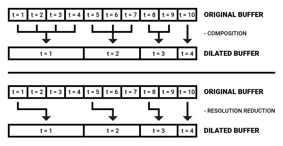
         Two methods for dimensionality reduction with dilated spectral buffers (in this figure unrolled for clarity).

By dilating each timestep in a new buffer by some ratio (such as an exponential incrementation of 2^t, for example) in proportion to the original buffer, the dimensionality can be drastically reduced while retaining a high resolution of spectral developments at the most recent timesteps. The values of the dilated buffer can either be obtained from the original buffer by simply looking up single values further and further back, but it is also possible to combine the number of timesteps to be collapsed by extracting the average or median spectrum across the duration.

The driving concept behind a dilated spectral buffer is to keep the most recent spectral impressions in memory while also retaining some information about the “big picture” context in an efficient way.

Below is a simplified code snippet for making dilated spectral frames using a Gammatone filterbank. Note that this example uses offline processing, but the filterbank can be applied real-time as well, inserting spectral frames to a circular buffer.

from gammatone import gtgram
import numpy as np

class GammatoneFilterbank:
    # Initialize Gammatone filterbank
    def __init__(self, 
                 sample_rate, 
                 window_time, 
                 hop_time, 
                 num_filters, 
                 cutoff_low):
        self.sample_rate = sample_rate
        self.window_time = window_time
        self.hop_time = hop_time
        self.num_filters = num_filters
        self.cutoff_low = cutoff_low
    # Make a spectrogram from a number of audio samples
    def make_spectrogram(self, audio_samples):
        return gtgram.gtgram(audio_samples,
                             self.sample_rate,
                             self.window_time,
                             self.hop_time,
                             self.num_filters,
                             self.cutoff_low)
    # Divide audio samples into dilated spectral buffers
    def make_dilated_spectral_frames(self, 
                                     audio_samples, 
                                     num_frames, 
                                     dilation_factor):
        spectrogram = self.make_spectrogram(audio_samples)
        spectrogram = np.swapaxes(spectrogram, 0, 1)
        dilated_frames = np.zeros((len(spectrogram), 
                                  num_frames, 
                                  len(spectrogram[0])))

        for i in range(len(spectrogram)):
            for j in range(num_frames):
                dilation = np.power(dilation_factor, j)

                if i - dilation < 0:
                    dilated_frames[i][j] = spectrogram[0]
                else:
                    dilated_frames[i][j] = spectrogram[i - dilation]

        return dilated_frames

 

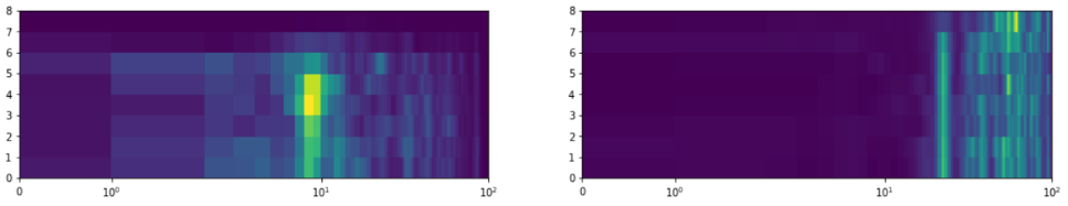
                            Result: Two examples of dilated spectral buffers visualized as a quadrilateral mesh.

Embedding the buffer

In many models of human memory, selective attention is applied after sensory memory as a filter to prevent overload of information in short-term memory [3]. Since humans have limited cognitive resources, it is advantageous to allocate attention to certain auditory sensations to optimize consumption of mental energy.

This process can be approached with an expansion of the autoencoder neural network architecture. Using this architecture, it’s possible to combine sensory memory of sounds with the bottleneck of selective attention by feeding it dilated frequency spectrum buffers for producing embeddings rather than feeding only the momentary frequency information. To cope with sequential information, a special type of architecture called a sequence-to-sequence autoencoder can be used [6].

Sequence-to-sequence (Seq2Seq) models typically use LSTM units to encode a sequence of data (an English sentence, for example) to an internal representation containing a compressed “meaning” about the sequence as a whole. This internal representation can then be decoded back into a sequence (the same sentence, but in Spanish, for example) [7].

A feature of embedding sounds in this way, is that it makes it possible to analyze and process them using simple feed-forward neural networks which are cheaper to run.

After training a network such as the one drawn below, the right half (the decoding part) can be “cut off”, thus generating a network for encoding temporal frequency information into a compressed space. Good results have been achieved in this area of research by Y. Chung et. al. with Audio Word2Vecwhich succeeded in generating embeddings describing the sequential phonetic structures of vocal recordings by applying a Seq2Seq autoencoder architecture [6]. With greater diversity of input data, it could also be possible to produce embeddings that describe sounds in a more general way.

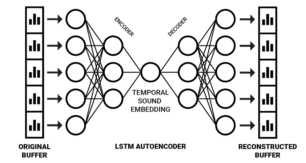
           A simplified illustration of a sequential autoencoder which produces temporal sound embeddings.

Listening with Keras

Using the approach described above, we can implement a Seq2Seq autoencoder with Keras to produce audio embeddings. I call this a ListenerNetwork, since its purpose is to “listen” to incoming sequences of sounds and reduce them to a more compact and meaningful representation which we can then analyze and process.

To train this network, ~3 hours of audio from the UrbanSound8K dataset were used. This dataset contains a selection of environmental sound clips divided into categories. The sounds were processed using a Gammatone filterbank and was segmented into dilated spectral buffers of 8 timesteps with 100 spectral filters each.

from keras.models import Model
from keras.layers import Input, LSTM, RepeatVector
def prepare_listener(timesteps,
                     input_dim,
                     latent_dim,
                     optimizer_type,
                     loss_type):
    """Prepares Seq2Seq autoencoder model

        Args:
            :param timesteps: The number of timesteps in sequence
            :param input_dim: The dimensions of the input
            :param latent_dim: The latent dimensionality of LSTM
            :param optimizer_type: The type of optimizer to use
            :param loss_type: The type of loss to use

        Returns:
            Autoencoder model, Encoder model
    """

    inputs = Input(shape=(timesteps, input_dim))
    encoded = LSTM(int(input_dim / 2), 
                   activation="relu", 
                   return_sequences=True)(inputs)
    encoded = LSTM(latent_dim, 
                   activation="relu", 
                   return_sequences=False)(encoded)
    decoded = RepeatVector(timesteps)(encoded)
    decoded = LSTM(int(input_dim / 2), 
                   activation="relu", 
                   return_sequences=True)(decoded)
    decoded = LSTM(input_dim, 
                   return_sequences=True)(decoded)

    autoencoder = Model(inputs, decoded)
    encoder = Model(inputs, encoded)

    autoencoder.compile(optimizer=optimizer_type, 
                        loss=loss_type,  
                        metrics=['acc'])

    return autoencoder, encoder

For my data, this code produces the network architecture below: 

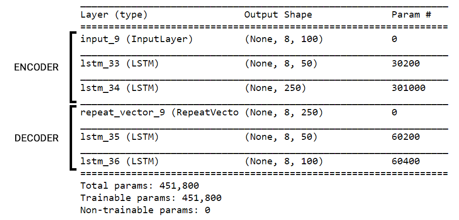
This Listener Network was trained using mean squared error and Adagrad optimization for 50 epochs on a NVIDIA GTX 1070 GPU arriving at a reconstruction accuracy of 42%. Training took a while so I stopped early, though progress did not seem to have stagnated yet. I’m very interested to see the performance of such a model with a larger dataset and more computational capacity for training.

There is certainly room for improvement here, but the images below show that the coarse structure of the sequences were captured after compressing the input by a factor of 3.2.

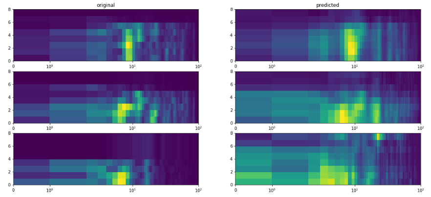
                 Some examples of original data and predictions by the autoencoder to illustrate reconstruction fidelity.

---

This was the second part of my article series on audio processing with neural networks. In the final article we will put the concepts to use in creating a network for analyzing audio embeddings.

Follow to stay updated and feel free to leave claps if you enjoyed the article!

To stay in touch, please feel free to connect with me on LinkedIn!

References

[1] J. J. Eggermont, “Between sound and perception: reviewing the search for a neural code.,” Hear. Res., vol. 157, no. 1–2, pp. 1–42, Jul. 2001.

[2] C. Alain, D. L. Woods, and R. T. Knight, “A distributed cortical network for auditory sensory memory in humans,” Brain Res., vol. 812, no. 1–2, pp. 23–37, Nov. 1998.

[3] A. Wingfield, “Evolution of Models of Working Memory and Cognitive Resources,” Ear Hear., vol. 37, p. 35S–43S, 2016.

[4] “Implementing Circular/Ring Buffer in Embedded C”, Embedjournal.com, 2014. [Online]. Available: https://embedjournal.com/implementing-circular-buffer-embedded-c/.

[5] A. Van Den Oord et al., “Wavenet: A Generative Model for Raw Audio.”

[6] Y.-A. Chung, C.-C. Wu, C.-H. Shen, H.-Y. Lee, and L.-S. Lee, “Audio Word2Vec: Unsupervised Learning of Audio Segment Representations Using Sequence-to-Sequence Autoencoder,” in Proceedings of the Annual Conference of the International Speech Communication Association, 2016, pp. 765–769.

[7] F. Chollet, “A ten-minute introduction to sequence-to-sequence learning in Keras”, Blog.keras.io, 2018. [Online]. Available: https://blog.keras.io/a-ten-minute-introduction-to-sequence-to-sequence-learning-in-keras.html.

音频相关文章的搬运工，如有侵权 请联系我们删除。

微博：砖瓦工-日记本

联系方式qq:1657250854