IC-Light：ICLR2025满分论文，ControlNet作者新作，控制光照，更自然地融合图片！

最新推荐文章于 2025-02-26 13:26:20 发布

Sherlock Ma

最新推荐文章于 2025-02-26 13:26:20 发布

阅读量2.8k

点赞数 23

分类专栏： AIGC 图像编辑 stable diffusion 文章标签：人工智能 ai 计算机视觉图像处理 AI作画 stable diffusion

本文链接：https://blog.csdn.net/sherlockMa/article/details/144189071

版权

AIGC 同时被 3 个专栏收录

30 篇文章

订阅专栏

图像编辑

4 篇文章

订阅专栏

stable diffusion

3 篇文章

订阅专栏

1.简介

在今年的ICLR会议上，一篇论文引起了极大的关注，因为它罕见地获得了四位审稿人同时给出的满分10分评价。如果这一评分能够持续到正式的录用通知，这将成为近五年来ICLR唯一的一篇满分论文。这篇论文的作者张吕敏，是业界广为人知的ControlNet的主要研究者。张吕敏在苏州大学完成了他的本科学业后，前往斯坦福大学继续他的博士学位研究。

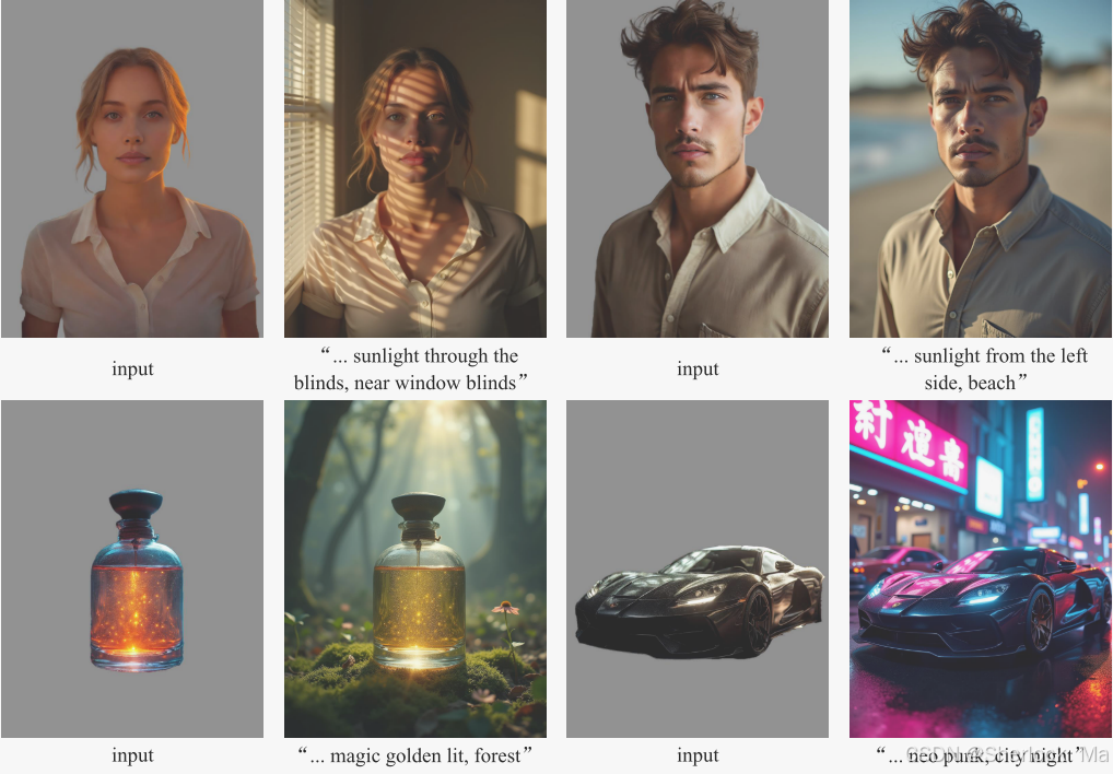
IC-Light（Imposing Consistent Light）是一种用于操控图像照明的技术。它通过捕捉背景图的光照信息来重新调整主体的光照，最后对整体图像进行微调，生成更加自然的图片。

IC-Light技术能够随心所欲地操纵照片中的光源和背景，巧妙地将主体、光源与背景三者迅速而无缝地融合于一张图像之中，呈现出令人赞叹的效果。

效果图：

论文审稿地址：Scaling In-the-Wild Training for Diffusion-based Illumination Harmonization and Editing by Imposing Consistent Light Transport | OpenReview

github地址：https://github.com/lllyasviel/IC-Light

Demo地址：https://huggingface.co/spaces/lllyasviel/IC-Light

第二代版本Demo地址：https://huggingface.co/spaces/lllyasviel/iclight-v2-vary

权重地址：https://huggingface.co/lllyasviel/ic-light/tree/main

2.效果展示

IC-Light具有两种工作流：

其中fc工作流是直接将人物从图像中抠出来，然后根据提示词生成一张新的照片。
fbc工作流允许我们导入指定的背景图，并且不会对其进行修改。

这里我只演示fc工作流

左图为原图，中间是主体抠图结果，右图是模型生成结果

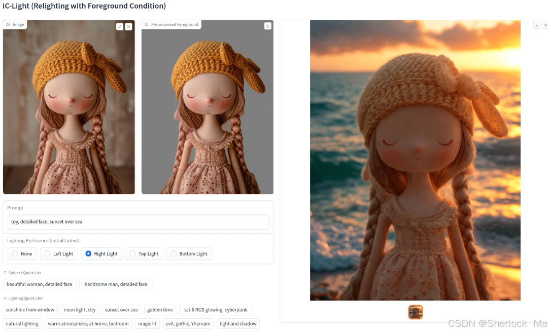
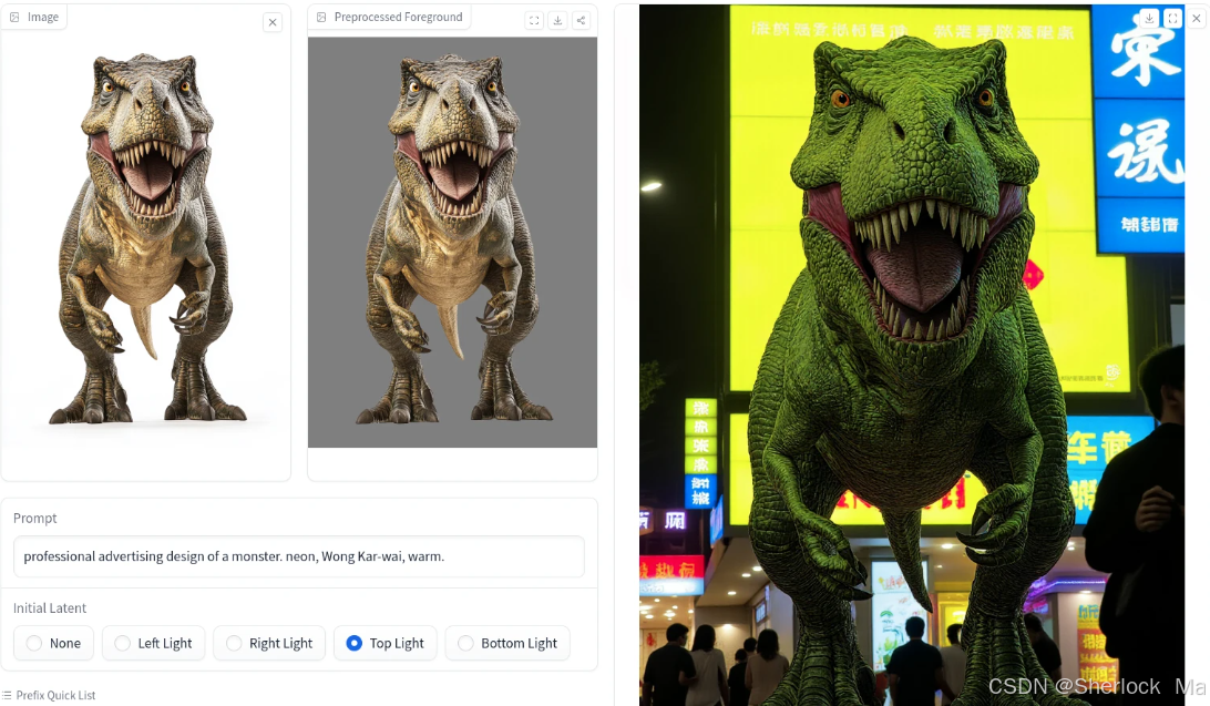
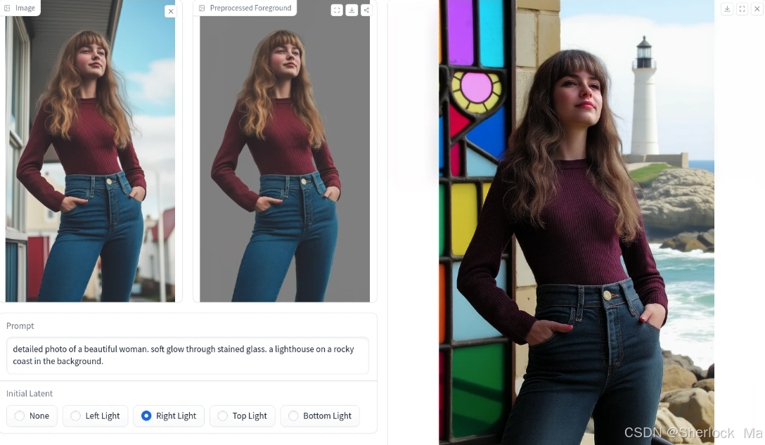
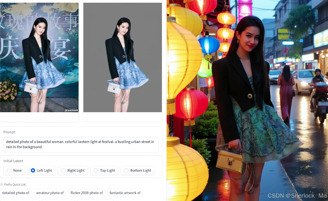
在我看来，效果已经非常令人满意。尽管在某些情况下人脸的渲染存在一些变化，但在光照表现上，它已经实现了与背景的无缝融合，达到了近乎完美的境界。

3.论文详解

Introduction

编辑图像中的光照是深度学习和图像编辑中的一项基本任务。经典的计算机图形方法通常使用物理照明模型来对图像的外观进行建模。

然而，在更大的尺度上训练具有更多多样性的照明编辑模型比看起来更具挑战性。

第一个挑战在于保持所需的模型行为，以确保正确的照明操作，而不是偏离到意外的随机行为。随着数据集大小和多样性的增加，学习目标的映射和分布可能变得模糊和不确定。在没有适当约束的情况下，训练可能产生结构引导的随机图像生成器，从而导致不与期望的照明编辑要求对准的输出。

第二个挑战是在修改照明时保留底层图像细节和固有属性，例如反射或反射颜色。由于扩散算法的随机性和潜在空间的编码-解码过程，基于扩散的图像生成器固有地倾向于将随机性引入图像内容，使得难以保留细粒度的细节。

在本文中，作者提出了一种在训练过程中施加一致光（IC光）传输的方法，该方法基于光传输独立性的物理原理-不同照明条件下物体外观的线性混合与混合照明下的外观一致。通过强制执行这种一致性，作者引入了一个强大的、物理根源的约束，确保模型只修改图像的照明方面，同时保留其他内在属性，如亮度和精细的图像细节。

Method

数据集构建

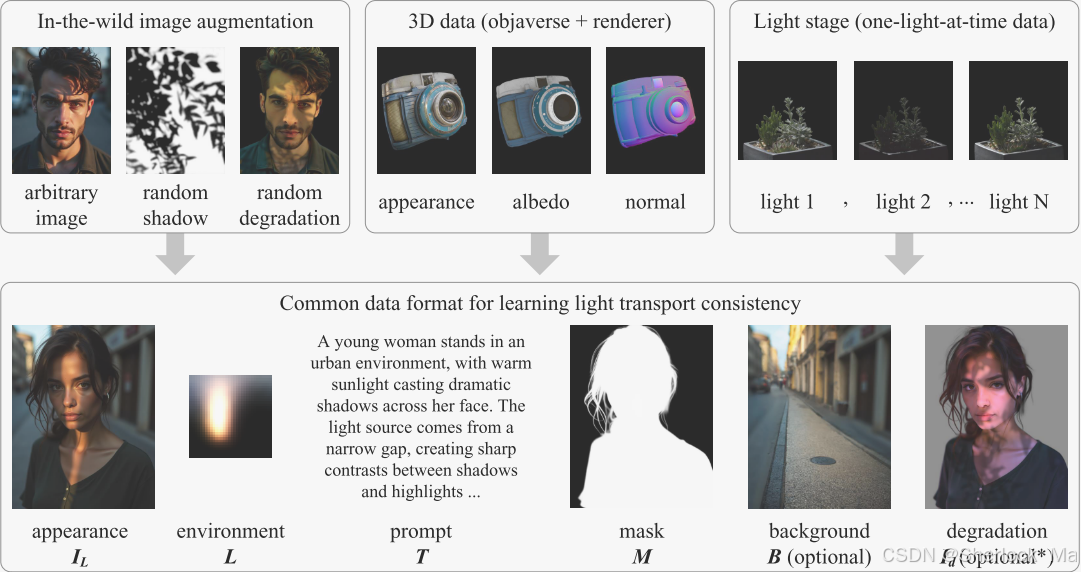
作者使用多种可用类型的数据源对照明效果的分布进行建模：任意图像，3d数据和灯光舞台(Light stage)图像。这些分布允许捕获多样化和复杂的现实世界照明场景，例如，背光、边缘光、辉光等。

为简单起见，我们将所有数据处理为通用格式。每个目标图像 $I_L \in R^{h\times w\times3}$ 与32 px环境光信息（environment maps） $L \in R^{32\times 32\times3}$ 、前景掩模 $M \in R^{h\times w}$ 、可选的背景图像 $B \in R^{h\times w\times3}$ 和可选的退化图像 $I_d \in R^{h\times w\times3}$ 配对。

对于普通图片 $I_L$ ：

使用Diffusionlight或自己的方法提取环境光信息L
使用RMBG-1.4检测前景掩模，得到M
并使用distill-accelerated Stable Diffusion生成背景图像，得到B
使用Florence-2检测提示词，或者如果图像来自文本图像数据集，则使用现有的图像提示，得到T。
然后生成一个“退化图像”，它与原图共享相同的主体内容，但已完全改变照明。具体来说，作者随机应用补充材料的6个亮度提取方法来提取图像的亮度。然后，使用3种随机法线估计方法合成软阴影图像，并使用随机阴影材料合成硬阴影。最后，我们添加一个随机水平的镜面反射随机区域。
- 阴影图像是从几个在线图像库存购买的20 k高质量阴影材料，以及使用Flux LoRA在这些20 k购买的样本上训练的500 k生成材料。接着作者通过比较CLIP Vision与关键词“美丽的灯光”、“灯光”和“照明”的相似度，过滤了50 M图像，最终确定了6 M图像

对于3D图像 $I_L$ ：

作者使用之前提取的环境光信息L。
这里作者不生成退化图像 $I_d$ ，而是直接使用随机的未配对环境光信息L去渲染物体，作为退化图像 $I_d$ 。作者数据集的这一部分的比例最终确定为400万张图像。

对于Light stage图像 $I_L$ ：

作者使用来自Mnichelson（2006），Liu等人（2024 a）的多个灯光舞台数据集，以及具有20 k灯光舞台外观的内部数据集。作者将所有One-Light-At-a-Time（OLAT）数据预渲染为上述相同的格式。
作者使用之前提取的环境光信息L渲染图像，作为退化图像 $I_d$ 。

这里做一个简单的总结：就是原来的高质量图片 $I_L$ ，提取主体掩码M和描述信息T，然后作者想办法加了点低质量内容（和原图不匹配的环境光信息L），生成了低质量的图片 $I_d$ 。

训练的时候，输入低质量图片 $I_d$ ，标签是高质量图片 $I_L$ 。

施加一致的光传输（IMPOSING CONSISTENT LIGHT TRANSPORT）

学习大规模，复杂和嘈杂的数据是具有挑战性的。如果没有合适的正则化和约束，模型很容易退化为与预期照明编辑不对应的随机行为。作者的解决方案是在训练过程中施加一致光（IMPOSING CONSISTENT LIGHT，即IC-Light）传输，其根源在于物理原理，即物体在不同照明条件下的外观的线性混合与其在混合照明条件下的外观一致。

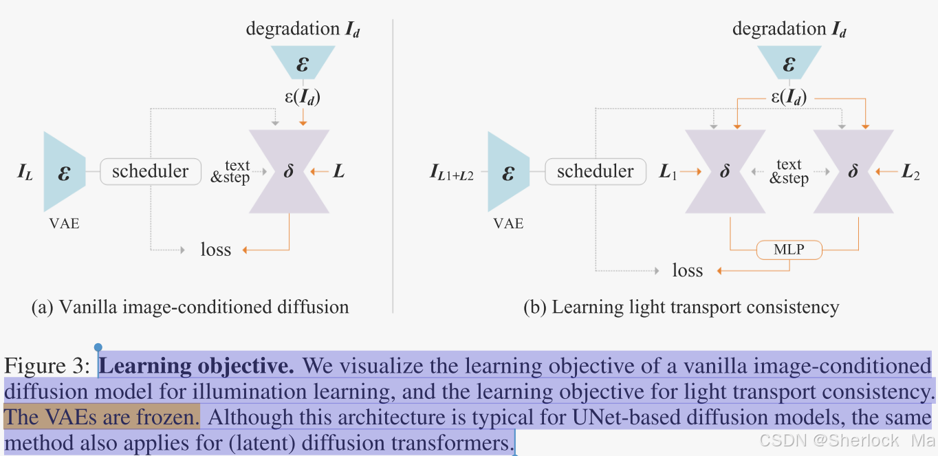
扩散模型的损失函数

作者从一个vanilla 扩散模型开始，在没有其他特殊约束的情况下学习光照。具体来说：

对于输入，作者将其输入层的卷积层通道数扩展至四个，以便更好地处理退化图像，即 $I_d$
对于环境光条件L，作者将HDRI环境光L reshape为长度3072的向量，并使用MLP（由Leaky Relu激活）将环境光转变为2304的向量，最后reshape为3 × 768的向量组（3个令牌，每个令牌768个通道）。这样SD就可以直接接收处理好的环境光嵌入作为其输入。
对于目标图像（高质量的原始图像） $I_L$ 首先将IL编码为潜图像 $\varepsilon (I_L)$ ，然后逐渐将噪声添加到潜图像以产生噪声潜图像 $\varepsilon (I_L)_t$ ，其中t表示添加噪声的次数。
对于网络δ，可以是流匹配模型，也可以是扩散模型。作用是通过退化图像 $I_d$ 和原始图像 $I_L$ 预测噪声 $\epsilon$ ，其损失函数如下： $L_{vanilla}=\left \| \epsilon -\delta (\varepsilon (I_L)_t,t,L,\varepsilon(I_d) )\right \|^2_2$

光传输一致性

在计算摄影中，光传输理论证明，对于任意外观 $I_L$ 和相关环境照明L，矩阵T总是存在，即 $I^*_L=TL$ ，其中*表示原始高动态范围（HDR）中的图像。

简单来说：如果我们知道物体在某些特定照明条件下的外观（L），我们可以通过这个线性模型来预测物体在其他照明条件下的外观（ $I^*_L$ ），而中间的转换条件T一定存在。

真实世界的测量证明了T总是可以用单个矩阵表示，而不需要任何非线性变换。由于这种线性，在单独的照明下物体外观的混合（例如，L1，L2）等同于合并照明下的外观（例如， $I^*_{L_1+L_2}$ ），即 $I^*_{L_1+L_2}=T(L_1+L_2)=I^*_{L_1}+I^*_{L_2}$

简单来说：如果我们知道物体在两个不同照明条件下的外观 $I^*_{L_1}$ 和 $I^*_{L_2}$ ，那么我们可以通过简单地将这两个外观相加，来预测物体在这两个照明条件合并时的外观 $I^*_{L_1+L_2}$ ，也就是说，补贴照明条件之间的信息是线性的。

光传输一致性的核心思想是保证 $I^*_{L_1+L_2}=T(L_1+L_2)=I^*_{L_1}+I^*_{L_2}$ ，以便将模型约束为仅修改图像照明而不改变其它固有属性（即保持内部光传输T不变）。但这只是理论，实际上还是有差异的，这就需要我们用网络去学习，我们可以通过最小化 $\left \| I^*_{L_1+L2} - (I^*_{L_1}+I^*_{L_2}) \right \|^2_2$ ，或者说最小化 $\left \| \epsilon _{L_1+L2} - (\epsilon _{L_1}+\epsilon _{L_2}) \right \|^2_2$ 来弥补差异。

实际上，作者使用一个简单的多层感知器 $\phi$ （MLP）来弥补差异： $\left \| \epsilon _{L_1+L2} -\phi (\epsilon _{L_1}+\epsilon _{L_2}) \right \|^2_2$

最后，加上前景掩码M，就是最终的损失函数： $L_{consistency}=\left \| M\odot (\epsilon _{L_1+L2} -\phi (\epsilon _{L_1}+\epsilon _{L_2})) \right \|^2_2$

总损失

$L=\lambda _{vanilla}L_{vanilla}+\lambda _{consistency}L_{consistency}$

其中L是合并目标，作者使用λvanilla = 1.0，λconsistency = 0.1作为默认权重

训练

作者采用了多阶段训练策略，分别训练模型的双流和单流部分，使用梯度冻结来冻结梯度图的某些部分。（这里作者没有明说，我感觉应该是第二阶段冻结diffusion模块 $\delta$ ，只训练MLP）

作者使用预定概率来平衡多个训练数据集。

在训练的初始阶段，普通图像数据和3D渲染数据以相等的概率出现。随着训练迭代的增加，每个批次中出现Light stage数据的概率增加。这使我们能够利用一小部分高质量的Light stage数据来提高最终模型的性能。

在训练的开始阶段，普通图像数据和3D数据的概率均为0.5，Light stage阶段为0.0。在100000次迭代后，将概率调整为普通图像数据的0.35，3D数据的0.35和Light stage数据的0.3。这些概率在整个训练过程中线性调整。

对于实验部分，请读者自行查看。

4.代码详解

环境搭建

新建虚拟环境，然后运行：

pip install torch torchvision --index-url https://download.pytorch.org/whl/cu121
pip install -r requirements.txt

使用方法

然后运行代码：

python gradio_demo.py

或者使用background-conditioned demo：

python gradio_demo_bg.py

模型架构

其中使用的模型如下：

sd15_name = 'stablediffusionapi/realistic-vision-v51'
tokenizer = CLIPTokenizer.from_pretrained(sd15_name, subfolder="tokenizer")
text_encoder = CLIPTextModel.from_pretrained(sd15_name, subfolder="text_encoder")
vae = AutoencoderKL.from_pretrained(sd15_name, subfolder="vae")
unet = UNet2DConditionModel.from_pretrained(sd15_name, subfolder="unet")
rmbg = BriaRMBG.from_pretrained("briaai/RMBG-1.4")

process_relight

上传图片并设置完提示词后，我们点击Relight，模型会运行process_relight()函数，这个函数包含了模型所有的步骤，具体来说：

调用 run_rmbg 函数（具体使用了BriaRMBG模型，‌它是一个由BRIA.AI公司开发的背景去除模型）去除输入图像的背景，返回处理后的前景图像input_fg和抠图掩码matting
process()：调用IC-Light模型处理光照信息
返回扣图结果和生成结果

@torch.inference_mode()
def process_relight(input_fg, prompt, image_width, image_height, num_samples, seed, steps, a_prompt, n_prompt, cfg, highres_scale, highres_denoise, lowres_denoise, bg_source):
    input_fg, matting = run_rmbg(input_fg)      # 调用 run_rmbg 函数去除输入前景图像的背景，返回处理后的前景图像input_fg和抠图掩码matting
    results = process(input_fg, prompt, image_width, image_height, num_samples, seed, steps, a_prompt, n_prompt, cfg, highres_scale, highres_denoise, lowres_denoise, bg_source)        # 调用模型进行处理
    return input_fg, results        # 返回扣图结果和生成结果

run_rmbg

这段代码定义了一个名为 run_rmbg 的函数，用于移除图像背景。具体步骤如下：

获取输入图像的形状，并确保其为三通道图像。
计算缩放因子 k，并根据 k 缩放图像。
将缩放后的图像转换为 PyTorch 张量，并传递给BriaRMBG模型进行背景移除。
对模型输出的 alpha 通道进行双线性插值，恢复到原始图像尺寸。
计算最终结果图像，并返回结果图像和 alpha 通道。

def run_rmbg(img, sigma=0.0):
    H, W, C = img.shape
    assert C == 3
    k = (256.0 / float(H * W)) ** 0.5       # 计算缩放因子 k
    feed = resize_without_crop(img, int(64 * round(W * k)), int(64 * round(H * k)))     # 根据 k 缩放图像,将图像缩放到新的尺寸。
    feed = numpy2pytorch([feed]).to(device=device, dtype=torch.float32)
    alpha = rmbg(feed)[0][0]        # 使用rmbg进行扣图，获取模型输出的 alpha 通道
    alpha = torch.nn.functional.interpolate(alpha, size=(H, W), mode="bilinear")    # 进行双线性插值，恢复到原始图像尺寸
    alpha = alpha.movedim(1, -1)[0]
    alpha = alpha.detach().float().cpu().numpy().clip(0, 1)
    result = 127 + (img.astype(np.float32) - 127 + sigma) * alpha       # 根据 alpha 通道和输入图像计算最终结果图像
    return result.clip(0, 255).astype(np.uint8), alpha      # 返回最终结果图像和 alpha 通道

process()

用于生成带有特定背景的图像。主要步骤如下：

获取光源类型：根据传入的bg_source参数确定背景光源类型。
选择背景：根据光源类型生成相应的背景图像
1. 如果无光源选择，下面选择t2i_pipe处理
2. 如果有光源，下面选择i2i_pipe
第一次去噪：将背景和前景图像拼接后转换为潜变量，并根据不同的背景类型选择t2i或i2i进行处理。
1. 第一次去噪的参数strength=lowres_denoise=0.9,num_inference_steps=int(round(steps / lowres_denoise)),
2. 第一次是在扩散模型的早期阶段，此时模型处理的是低分辨率的图像。这个阶段的目的是快速生成图像的大致轮廓和基本结构，而不关注细节。
解码图像，再还原回潜变量（相当于放大图像）
第二次去噪：将第一次去噪的结果和前景图像一起输入i2i_pipe，进行去噪
1. 无论有没有光照，一定使用i2i_pipe
2. 第二次去噪的参数strength=highres_denoise=0.5,num_inference_steps=int(round(steps / highres_denoise)),
3. 第一次是在模型的后期阶段使用，此时模型处理的是高分辨率的图像。这个阶段的目的是细化图像，恢复细节和纹理，使图像更加清晰和真实。
解码潜变量，最终生成最终图像。

完整代码如下：

@torch.inference_mode()
def process(input_fg, prompt, image_width, image_height, num_samples, seed, steps, a_prompt, n_prompt, cfg, highres_scale, highres_denoise, lowres_denoise, bg_source):
    # 1.获取光源类型
    bg_source = BGSource(bg_source)     # 获取光源类型
    input_bg = None

    # 2.根据光源类型选择背景
    if bg_source == BGSource.NONE:      # 根据光源类型选择背景
        pass
    elif bg_source == BGSource.LEFT:
        gradient = np.linspace(255, 0, image_width)     # 生成渐变数组
        image = np.tile(gradient, (image_height, 1))        # 将渐变数组在宽度方向上重复 image_width 次，形成一个二维数组。
        input_bg = np.stack((image,) * 3, axis=-1).astype(np.uint8)     #  将二维数组在通道维度上堆叠3次，形成一个三维数组
    elif bg_source == BGSource.RIGHT:
        gradient = np.linspace(0, 255, image_width)
        image = np.tile(gradient, (image_height, 1))
        input_bg = np.stack((image,) * 3, axis=-1).astype(np.uint8)
    elif bg_source == BGSource.TOP:
        gradient = np.linspace(255, 0, image_height)[:, None]
        image = np.tile(gradient, (1, image_width))
        input_bg = np.stack((image,) * 3, axis=-1).astype(np.uint8)
    elif bg_source == BGSource.BOTTOM:
        gradient = np.linspace(0, 255, image_height)[:, None]
        image = np.tile(gradient, (1, image_width))
        input_bg = np.stack((image,) * 3, axis=-1).astype(np.uint8)
    else:
        raise 'Wrong initial latent!'

    rng = torch.Generator(device=device).manual_seed(int(seed))     # 使用指定的种子初始化随机数生成器

    # 3.第一次去噪
    # 生成前景的潜变量concat_conds，这里的前景fg是BGSource.NONE时当背景用的(也就相当于背景)
    fg = resize_and_center_crop(input_fg, image_width, image_height)    # 调整输入前景图像的大小并居中裁剪
    concat_conds = numpy2pytorch([fg]).to(device=vae.device, dtype=vae.dtype)
    concat_conds = vae.encode(concat_conds).latent_dist.mode() * vae.config.scaling_factor  # 将前景图像转换为潜变量

    conds, unconds = encode_prompt_pair(positive_prompt=prompt + ', ' + a_prompt, negative_prompt=n_prompt)     # 文本提示编码：将正向和负向提示编码为嵌入向量，并通过重复，使正负提示词数量一样

        if input_bg is None:        # 4.1  bg_source == BGSource.NONE时，背景为空
        latents = t2i_pipe(
            prompt_embeds=conds,
            negative_prompt_embeds=unconds,
            width=image_width,
            height=image_height,
            num_inference_steps=steps,
            num_images_per_prompt=num_samples,
            generator=rng,
            output_type='latent',
            guidance_scale=cfg,
            cross_attention_kwargs={'concat_conds': concat_conds},      # 前景
        ).images.to(vae.dtype) / vae.config.scaling_factor
    else:       # 4.2  bg_source ！= BGSource.NONE时，也就是有其他背景时
        bg = resize_and_center_crop(input_bg, image_width, image_height)
        bg_latent = numpy2pytorch([bg]).to(device=vae.device, dtype=vae.dtype)
        bg_latent = vae.encode(bg_latent).latent_dist.mode() * vae.config.scaling_factor    # 背景生成潜变量[b,4,潜w,潜h]=[b,4,96,64] (hw不固定)
        latents = i2i_pipe(         # [b,4,潜w,潜h]=[b,4,96,64] (hw不固定)
            image=bg_latent,        # 背景
            strength=lowres_denoise,
            prompt_embeds=conds,
            negative_prompt_embeds=unconds,
            width=image_width,
            height=image_height,
            num_inference_steps=int(round(steps / lowres_denoise)),
            num_images_per_prompt=num_samples,
            generator=rng,
            output_type='latent',
            guidance_scale=cfg,
            cross_attention_kwargs={'concat_conds': concat_conds},      # 前景
        ).images.to(vae.dtype) / vae.config.scaling_factor

    pixels = vae.decode(latents).sample     # 解码 [b,3,w,h]=[b,3,768,512] (hw不固定)
    pixels = pytorch2numpy(pixels)
    pixels = [resize_without_crop(
        image=p,
        target_width=int(round(image_width * highres_scale / 64.0) * 64),
        target_height=int(round(image_height * highres_scale / 64.0) * 64))     # [放大的w,放大的h,3] = [1152,768,3] (hw不固定)
    for p in pixels]        # 还原回原尺寸

    pixels = numpy2pytorch(pixels).to(device=vae.device, dtype=vae.dtype)
    latents = vae.encode(pixels).latent_dist.mode() * vae.config.scaling_factor     # 生成潜变量[1,4,潜w,潜h]=[1,4,144,96] (注意这里的潜变量相对于上面的潜变量，变大了，因为上面进行了缩放)
    latents = latents.to(device=unet.device, dtype=unet.dtype)

    image_height, image_width = latents.shape[2] * 8, latents.shape[3] * 8


    # 4.第二次去噪
    fg = resize_and_center_crop(input_fg, image_width, image_height)        # [放大的w,放大的h,3] = [1152,768,3] (hw不固定)
    concat_conds = numpy2pytorch([fg]).to(device=vae.device, dtype=vae.dtype)
    concat_conds = vae.encode(concat_conds).latent_dist.mode() * vae.config.scaling_factor  # 生成潜变量[1,4,潜w,潜h]=[1,4,144,96]

    latents = i2i_pipe(     # [1,4,144,96]
        image=latents,      # 第一次去噪的结果
        strength=highres_denoise,
        prompt_embeds=conds,
        negative_prompt_embeds=unconds,
        width=image_width,
        height=image_height,
        num_inference_steps=int(round(steps / highres_denoise)),
        num_images_per_prompt=num_samples,
        generator=rng,
        output_type='latent',
        guidance_scale=cfg,
        cross_attention_kwargs={'concat_conds': concat_conds},      # 前景
    ).images.to(vae.dtype) / vae.config.scaling_factor

    pixels = vae.decode(latents).sample     # 解码潜变量 [1,3,1152,768]

    return pytorch2numpy(pixels)

接下来，我们对里面的每个部分进行详细解读

光源类型及背景光源图生成

BGSource如下：

class BGSource(Enum):
    NONE = "None"
    LEFT = "Left Light"
    RIGHT = "Right Light"
    TOP = "Top Light"
    BOTTOM = "Bottom Light"

接着根据光源类型，在步骤二中会生成对应的input_bg，

# 2.根据光源类型选择背景
if bg_source == BGSource.NONE:      # 根据光源类型选择背景
    pass
elif bg_source == BGSource.LEFT:
    gradient = np.linspace(255, 0, image_width)     # 生成渐变数组
    image = np.tile(gradient, (image_height, 1))        # 将渐变数组在宽度方向上重复 image_width 次，形成一个二维数组。
    input_bg = np.stack((image,) * 3, axis=-1).astype(np.uint8)     #  将二维数组在通道维度上堆叠3次，形成一个三维数组
elif bg_source == BGSource.RIGHT:
    gradient = np.linspace(0, 255, image_width)
    image = np.tile(gradient, (image_height, 1))
    input_bg = np.stack((image,) * 3, axis=-1).astype(np.uint8)
elif bg_source == BGSource.TOP:
    gradient = np.linspace(255, 0, image_height)[:, None]
    image = np.tile(gradient, (1, image_width))
    input_bg = np.stack((image,) * 3, axis=-1).astype(np.uint8)
elif bg_source == BGSource.BOTTOM:
    gradient = np.linspace(0, 255, image_height)[:, None]
    image = np.tile(gradient, (1, image_width))
    input_bg = np.stack((image,) * 3, axis=-1).astype(np.uint8)
else:
    raise 'Wrong initial latent!'

部分背景可视化结果如下：

bg_source == BGSource.LEFT

bg_source == BGSource.RIGHT

可见，其生成的背景是根据光照方向的反方向来的，列如，如果光照方向是右，那么背景图的方向是从左到右逐渐变暗。

可能的原因（个人猜想）：

扩散模型需要能够处理包括镜面反射在内的复杂照明效果，以便在图像生成和编辑中实现精确的照明操纵。
在某些情况下，背景的亮度变化可能与光照方向相反，是因为光线在到达相机之前经过了多次反射和散射。例如，当光线从一个方向照射到一个表面，然后反射到另一个方向时，可能会在背景上形成与原始光照方向相反的亮度变化。
在技术实现上，让背景的亮度变化与光照方向相反可能是为了简化计算或者利用特定的算法优势。例如，在某些图像合成技术中，通过反向亮度变化可以更容易地实现前景和背景的融合。

i2i_pipe

process()中调用i2i_pipe的部分如下：

latents = i2i_pipe(         # [b,4,潜w,潜h]=[b,4,96,64] (hw不固定)
    image=bg_latent,
    strength=lowres_denoise,    # 第一次去噪是0.9，第二次是0.5
    prompt_embeds=conds,
    negative_prompt_embeds=unconds,
    width=image_width,
    height=image_height,
    num_inference_steps=int(round(steps / lowres_denoise)),
    num_images_per_prompt=num_samples,
    generator=rng,
    output_type='latent',
    guidance_scale=cfg,
    cross_attention_kwargs={'concat_conds': concat_conds},
).images.to(vae.dtype) / vae.config.scaling_factor

具体来说，i2i_pipe会运行pipeline_stable_diffusion_img2img.py下的StableDiffusionImg2ImgPipeline类的__call__()方法，方法过程如下：

参数检查：确保输入参数符合预期，例如 prompt 和 image 是否有效。
编码提示词：将文本提示和负提示转换为嵌入向量（实际上啥也没做，作者在外部已经处理过了，这里只是走个流程）
预处理图像：对输入图像进行预处理（实际上啥也没做，作者在外部已经处理过了，这里只是走个流程）
设置时间步：根据 num_inference_steps 和 strength 确定时间步。
准备潜在变量：初始化潜在变量，用于后续的去噪过程。
准备额外步骤：准备额外的步骤参数，如 eta 和 generator。
去噪循环：通过迭代逐步去噪，生成最终图像。每一步都可能调用回调函数。
后处理：解码潜在变量，运行安全检查，处理输出格式，确保输出符合预期。
返回结果：返回生成的图像和是否包含不安全内容的标志。

预处理

这里的目的是处理提示词和图像，因为在外部已经处理过了，所以这里只是走了else直接返回了，

1-3步没什么重要的内容，我这里就直接略过了。唯一需要注意的地方是，这里会把正负提示词concat起来，放入prompt_embeds：

if self.do_classifier_free_guidance:    # [2b,len,c]
    prompt_embeds = torch.cat([negative_prompt_embeds, prompt_embeds])

时间步处理

用于生成时间步tensor

# 5. set timesteps      设置时间步
timesteps, num_inference_steps = retrieve_timesteps(        # timesteps=[999-0]共num_inference_steps个
    self.scheduler, num_inference_steps, device, timesteps, sigmas
)
timesteps, num_inference_steps = self.get_timesteps(num_inference_steps, strength, device)  # num_inference_steps=num_inference_steps*strength， timesteps=[999-0]共num_inference_steps个
latent_timestep = timesteps[:1].repeat(batch_size * num_images_per_prompt)      # timesteps[0]

如果步长设置为25，第一行的timesteps值如下，长度为28：

tensor([999, 972, 943, 913, 881, 848, 812, 774, 733, 689, 642, 592, 537, 479,
        418, 354, 290, 228, 171, 123,  83,  53,  32,  17,   9,   4,   1,   0],
       device='cuda:0')

如果步长设置为25，最终的timesteps值如下，长度为28*0.9=25（将长度变为原长度*strength）：

tensor([913, 881, 848, 812, 774, 733, 689, 642, 592, 537, 479, 418, 354, 290,
        228, 171, 123,  83,  53,  32,  17,   9,   4,   1,   0],
       device='cuda:0')

其中，retrieve_timesteps()核心部分如下：

scheduler.set_timesteps(num_inference_steps, device=device, **kwargs)
timesteps = scheduler.timesteps

其中，get_timesteps()代码部分如下，就是将原长度变为长度*strength，第一次去噪的值默认为strength=0.9：

def get_timesteps(self, num_inference_steps, strength, device):
    # get the original timestep using init_timestep
    init_timestep = min(int(num_inference_steps * strength), num_inference_steps)

    t_start = max(num_inference_steps - init_timestep, 0)
    timesteps = self.scheduler.timesteps[t_start * self.scheduler.order :]
    if hasattr(self.scheduler, "set_begin_index"):
        self.scheduler.set_begin_index(t_start * self.scheduler.order)

    return timesteps, num_inference_steps - t_start

生成噪声

latents = self.prepare_latents(
    image,
    latent_timestep,
    batch_size,
    num_images_per_prompt,
    prompt_embeds.dtype,
    device,
    generator,      # torch.Generator，process()定义
)

下面是其中的核心部分，具体来说，作者使用randn_tensor生成了随机噪声noise，再使用scheduler将噪声noise添加到原图init_latents上，返回init_latents。

init_latents = torch.cat([init_latents], dim=0)    # 图像
noise = randn_tensor(shape, generator=generator, device=device, dtype=dtype)

# get latents
init_latents = self.scheduler.add_noise(init_latents, noise, timestep)      # 在初始化潜在变量 init_latents 中添加噪声 noise，并指定时间步 timestep
latents = init_latents

其中noise 是使用 generator 作为随机数生成器，利用torch.randn()生成指定形状的随机张量（latents）

latents = torch.randn(shape, generator=generator, device=rand_device, dtype=dtype, layout=layout).to(device)    # 使用 generator 作为随机数生成器，生成指定形状的随机张量（latents），并将其移动到指定设备上。

去噪

去噪过程就是根据生成的噪声和时间步，使用u-net逐步去噪。

# 8. Denoising loop
num_warmup_steps = len(timesteps) - num_inference_steps * self.scheduler.order
self._num_timesteps = len(timesteps)
with self.progress_bar(total=num_inference_steps) as progress_bar:
    for i, t in enumerate(timesteps):
        if self.interrupt:
            continue

        # expand the latents if we are doing classifier free guidance
        latent_model_input = torch.cat([latents] * 2) if self.do_classifier_free_guidance else latents      # [2b,4,w,h]
        latent_model_input = self.scheduler.scale_model_input(latent_model_input, t)

        # predict the noise residual  预测噪声
        noise_pred = self.unet(
            latent_model_input,
            t,
            encoder_hidden_states=prompt_embeds,
            timestep_cond=timestep_cond,
            cross_attention_kwargs=self.cross_attention_kwargs,
            added_cond_kwargs=added_cond_kwargs,
            return_dict=False,
        )[0]        # [2b,4,w,h]

        # perform guidance
        if self.do_classifier_free_guidance:
            noise_pred_uncond, noise_pred_text = noise_pred.chunk(2)
            noise_pred = noise_pred_uncond + self.guidance_scale * (noise_pred_text - noise_pred_uncond)

        # compute the previous noisy sample x_t -> x_t-1  把噪声删掉
        latents = self.scheduler.step(noise_pred, t, latents, **extra_step_kwargs, return_dict=False)[0]

        ...

u-net网络结构

处理时间

将时间嵌入成一个1280维度的向量

# 1. time
t_emb = self.get_time_embed(sample=sample, timestep=timestep)   # [2b]=[2]->[2b,c]=[2,320]
emb = self.time_embedding(t_emb, timestep_cond)         # [2b,c]=[2,320]->[2b,1280]

处理提示词和图片隐空间向量

分别处理图像和文本信息。

encoder_hidden_states = self.process_encoder_hidden_states(     # 正负提示词    # [2b,len,768]encoder_hidden_states
    encoder_hidden_states=encoder_hidden_states, added_cond_kwargs=added_cond_kwargs
        )
sample = self.conv_in(sample)   # 卷积 [2b,8,w,h]->[2b,320,w,h]

U形网络去噪

U-Net网络结构大家应该很熟悉了，就是一个下采样+中间层+上采样的过程，我这里就不展示具体的模块了：

对于上采样，整体架构是3个CrossAttnDownBlock2D（其中2个Transformer层+2个ResnetBlock2D+1个卷积层）+1个DownBlock2D（ResnetBlock2D），
中间层只有1个CrossAttnDownBlock2D。
对于下采样，整体架构是3个CrossAttnDownBlock2D（其中2个Transformer层+2个ResnetBlock2D+1个卷积层）+1个DownBlock2D（ResnetBlock2D），

这里需要注意的是，在进入u-net网络之前，会经过一个叫hooked_unet_forward()的函数，这个函数的目的是将sample和cross_attention_kwargs以第1维度拼接起来（channel维度），变为原channel的两倍，而输入到u-net的cross_attention_kwargs变为空。相当于做了一次特征融合。

对于第一个i2i，sample是背景图，而原cross_attention_kwargs是前景图
对于第二个i2i，sample是i2i_pipe生成的结果，而原cross_attention_kwargs是前景图

def hooked_unet_forward(sample, timestep, encoder_hidden_states, **kwargs):
    c_concat = kwargs['cross_attention_kwargs']['concat_conds'].to(sample)
    c_concat = torch.cat([c_concat] * (sample.shape[0] // c_concat.shape[0]), dim=0)        # 根据 sample 的批量大小，重复 c_concat，使其与 sample 的批量大小匹配。
    new_sample = torch.cat([sample, c_concat], dim=1)   # 将 sample 和 c_concat 在通道维度上进行拼接，生成新的 new_sample。
    kwargs['cross_attention_kwargs'] = {}
    return unet_original_forward(new_sample, timestep, encoder_hidden_states, **kwargs)

tranformer block

j接下来我们再来详细说说CrossAttnDownBlock2D里面的TransformerBlock，以下是transformer的结构，可以看到就是里面有两个注意力模块，一个是图片的自注意力，另一个是图片提供Q，文本提供KV的cross-attention。其他部分和普通transformer完全一样。

@maybe_allow_in_graph
class BasicTransformerBlock(nn.Module)
    def forward(...) -> torch.Tensor:
        # 0. Self-Attention
        ...

        attn_output = self.attn1(       # 图像自注意力
            norm_hidden_states,
            encoder_hidden_states=encoder_hidden_states if self.only_cross_attention else None,
            attention_mask=attention_mask,
            **cross_attention_kwargs,
        )

        hidden_states = attn_output + hidden_states     # 残差连接
        
        # 3. Cross-Attention
        ...

        attn_output = self.attn2(       # cross-attention,图像提供Q，text提供K，V
                norm_hidden_states,
                encoder_hidden_states=encoder_hidden_states,
                attention_mask=encoder_attention_mask,
                **cross_attention_kwargs,
            )
            hidden_states = attn_output + hidden_states     # 残差连接

        # 4. Feed-forward
        if self.norm_type == "ada_norm_continuous":
            norm_hidden_states = self.norm3(hidden_states, added_cond_kwargs["pooled_text_emb"])
        elif not self.norm_type == "ada_norm_single":       # 默认走这里
            norm_hidden_states = self.norm3(hidden_states)

        ...

        if self._chunk_size is not None:
            # "feed_forward_chunk_size" can be used to save memory
            ff_output = _chunked_feed_forward(self.ff, norm_hidden_states, self._chunk_dim, self._chunk_size)
        else:
            ff_output = self.ff(norm_hidden_states)     # 默认走这里

        ...

        hidden_states = ff_output + hidden_states       # 残差连接
        if hidden_states.ndim == 4:
            hidden_states = hidden_states.squeeze(1)

        return hidden_states

后处理

后处理主要内容是使用 do_denormalize 列表作为参数，对图像进行反归一化处理。

if has_nsfw_concept is None:
    do_denormalize = [True] * image.shape[0]    # 全True
else:
    do_denormalize = [not has_nsfw for has_nsfw in has_nsfw_concept]

image = self.image_processor.postprocess(image, output_type=output_type, do_denormalize=do_denormalize)     # 反归一化[b,4,w,h]

第一次和第二次之间还原尺寸

这里的操作就是把第一次生成的隐空间向量转回正常空间，然后放大，然后又转回隐空间，接着进行第二次去噪。

pixels = vae.decode(latents).sample     # 解码 [b,3,w,h]=[b,3,768,512] (hw不固定)
pixels = pytorch2numpy(pixels)
pixels = [resize_without_crop(
    image=p,
    target_width=int(round(image_width * highres_scale / 64.0) * 64),
    target_height=int(round(image_height * highres_scale / 64.0) * 64))     # [放大的w,放大的h,3] = [1152,768,3] (hw不固定)
for p in pixels]        # 放大，还原回原尺寸

pixels = numpy2pytorch(pixels).to(device=vae.device, dtype=vae.dtype)
latents = vae.encode(pixels).latent_dist.mode() * vae.config.scaling_factor     # 生成潜变量[1,4,潜w,潜h]=[1,4,144,96] (注意这里的潜变量相对于上面的潜变量，变大了，因为上面进行了缩放)
latents = latents.to(device=unet.device, dtype=unet.dtype)

t2i_pipe

在处理背景图时，光源为None时，调用的是t2i_pipe，而光源非None时，调用的是i2i_pipe。

区别：

t2i不输入图像，也就是说t2i输入到UNet的噪声是纯噪声，而i2i输入到UNet里面的是含有背景或前景信息的噪声。(详见上文生成噪声部分及下文生成噪声部分)
t2i没有strength调整步长

latents = t2i_pipe(
    prompt_embeds=conds,
    negative_prompt_embeds=unconds,
    width=image_width,
    height=image_height,
    num_inference_steps=steps,
    num_images_per_prompt=num_samples,
    generator=rng,
    output_type='latent',
    guidance_scale=cfg,
    cross_attention_kwargs={'concat_conds': concat_conds},
).images.to(vae.dtype) / vae.config.scaling_factor

生成噪声

t2i的prepare_latents()方法如下，可见它是纯噪声的生成，没有引入图像信息

def prepare_latents(self, batch_size, num_channels_latents, height, width, dtype, device, generator, latents=None):
    ...

    if latents is None:
        latents = randn_tensor(shape, generator=generator, device=device, dtype=dtype)
    else:
        latents = latents.to(device)

    # scale the initial noise by the standard deviation required by the scheduler
    latents = latents * self.scheduler.init_noise_sigma
    return latents