networkx构建delaunay图，并根据节点坐标绘制图

from libpysal import weights, examples
from libpysal.cg import voronoi_frames
from contextily import add_basemap
import matplotlib.pyplot as plt
import networkx as nx
import numpy as np
import geopandas
import itertools

# 输入数据
cases = geopandas.read_file(r"E:\code_practice\gitee\Python地理空间分析指南\nx_study\networkx\examples\geospatial\cholera_cases.gpkg")
cases

	Id	Count	geometry
0	0	1	POINT (-15539.921 6712903.938)
1	0	3	POINT (-15356.721 6712858.073)
2	0	2	POINT (-15336.090 6712866.374)
3	0	1	POINT (-15353.877 6713017.559)
4	0	0	POINT (-15282.597 6712895.684)
...	...	...	...
319	0	0	POINT (-14951.181 6712211.606)
320	0	0	POINT (-14979.678 6712225.369)
321	0	3	POINT (-15591.770 6712227.697)
322	0	0	POINT (-15525.087 6712152.522)
323	0	0	POINT (-14952.725 6712116.692)

324 rows × 3 columns

• 为了让nx正确绘制图的节点，我们需要为数据集中的每个点构造坐标数组
• 从geometry列中提取x,y坐标

# x坐标
x = cases.geometry.x
x

0     -15539.921064
1     -15356.720566
2     -15336.089980
3     -15353.877335
4     -15282.596809
           ...     
319   -14951.180762
320   -14979.678278
321   -15591.770010
322   -15525.086590
323   -14952.725267
Length: 324, dtype: float64

# y
y= cases.geometry.y
y

0      6.712904e+06
1      6.712858e+06
2      6.712866e+06
3      6.713018e+06
4      6.712896e+06
           ...     
319    6.712212e+06
320    6.712225e+06
321    6.712228e+06
322    6.712153e+06
323    6.712117e+06
Length: 324, dtype: float64

nodes_coords = np.column_stack((x,y))
#切片展示
nodes_coords[:5]

array([[ -15539.92106438, 6712903.93781305],
       [ -15356.72056559, 6712858.07280407],
       [ -15336.08997978, 6712866.3743291 ],
       [ -15353.877335  , 6713017.55898743],
       [ -15282.5968086 , 6712895.68378701]])

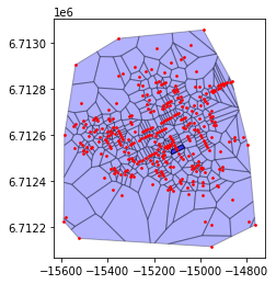
• 泰森多边形的建立 (具体看libpysal库)
• 并将

region_df, point_df  = voronoi_frames(nodes_coords, clip="convex hull")
fig, ax = plt.subplots()
region_df.plot(ax=ax, color='blue',edgecolor='black', alpha=0.3)
point_df.plot(ax=ax, color='red',markersize =3)

<AxesSubplot:>

• 利用泰森多边形，可以利用“rook”临接性来构造他们之间的邻接图
• 如果泰森多边形共享边/面，则它们是相邻的

delaunay = weights.Rook.from_dataframe(region_df)
delaunay_graph = delaunay.to_networkx()
nx.draw(delaunay_graph,node_size =10)

# 给节点匹配coords
positions = dict(zip(delaunay_graph.nodes, nodes_coords))
#切片展示
positions_head = dict(itertools.islice(positions.items(), 5))
positions_head

{0: array([ -15539.92106438, 6712903.93781305]),
 1: array([ -15356.72056559, 6712858.07280407]),
 2: array([ -15336.08997978, 6712866.3743291 ]),
 3: array([ -15353.877335  , 6713017.55898743]),
 4: array([ -15282.5968086 , 6712895.68378701])}

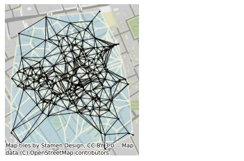
• add_basemap :获取地理底图
• positions ：dict，节点-坐标，用于可视化

# 可视化
# 用nx可视化delaunay_graph,并展示节点正确的地理位置
ax = region_df.plot(facecolor="lightblue", alpha=0.50, edgecolor="cornsilk", linewidth=2)
add_basemap(ax)
ax.axis("off")
nx.draw(
    delaunay_graph,
    positions,   #以节点为键，坐标为值
    ax=ax,
    node_size=2,
    node_color="k",
    edge_color="k",
    alpha=0.8,
)
plt.show()

#下面是直接用点、多边形数据可视化的结果，可以与上面对比一下
region_df, point_df  = voronoi_frames(nodes_coords, clip="convex hull")
fig, ax = plt.subplots()
region_df.plot(ax=ax, color='blue',edgecolor='black', alpha=0.3)
point_df.plot(ax=ax, color='red',markersize =3)

<AxesSubplot:>