


1.根据一组lines构建graph
- 教程数据来源,基础数据都在nx.example文件夹中
- 官方教程
- 从lines创建graph通常有两种方法
- 方法1:原始法(primal approach),每个交叉点是一个节点
- 方法2: 对偶法(dual approach),每条线都是一个节点,相交拓扑被转换为边
import geopandas as gpd
import matplotlib.pyplot as plt
import momepy
import networkx as nx
from contextily import add_basemap
from libpysal import weights
import itertools
1读取rivers数据(一组line),构造primal graph
1.1读取数据
rivers = gpd.read_file(r"E:\code_practice\gitee\Python地理空间分析指南\nx_study\networkx\examples\geospatial\rivers.geojson")
rivers.head()
| Length | id | geometry | |
|---|---|---|---|
| 0 | 8726.582 | 0 | LINESTRING (554143.903 9370463.606, 554090.774... |
| 1 | 4257.036 | 1 | LINESTRING (556297.090 9365917.050, 555900.606... |
| 2 | 4126.414 | 2 | LINESTRING (556950.010 9367879.530, 556969.360... |
| 3 | 1193.850 | 3 | LINESTRING (557295.943 9363890.831, 557179.526... |
| 4 | 3678.113 | 4 | LINESTRING (557237.735 9362710.787, 557322.402... |
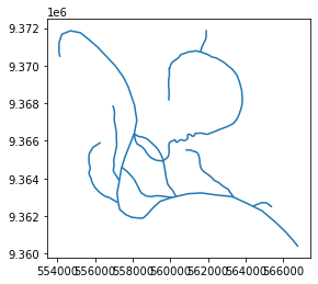
rivers.plot()
<AxesSubplot:>
1.2构造primal graph
- momepy 将gdf 转为graph
# 构造原始图
G = momepy.gdf_to_nx(rivers)
nx.draw(G,node_size = 10)
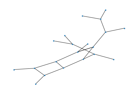
- 看一下G中的节点和边信息
- 每个节点的编号类型是tuple,值为坐标值
# 节点信息展示方法1:
G.nodes()(data= True)
NodeDataView({(554143.9027843038, 9370463.606285565): {'nodeID': 0}, (558080.5283343233, 9366376.590186208): {'nodeID': 1}, (556297.0900288569, 9365917.049970472): {'nodeID': 2}, (557237.7347526932, 9362710.78680345): {'nodeID': 3}, (556950.0100390166, 9367879.529990936): {'nodeID': 4}, (557295.9432376046, 9363890.830840945): {'nodeID': 5}, (560098.0373490807, 9362989.473788045): {'nodeID': 6}, (557427.1586279813, 9364610.527111784): {'nodeID': 7}, (559631.0745073119, 9364934.686608903): {'nodeID': 8}, (561623.109724192, 9370725.055553077): {'nodeID': 9}, (560319.5985694304, 9363042.402333023): {'nodeID': 10}, (559897.2550022183, 9369874.224961167): {'nodeID': 11}, (559964.2083513336, 9369823.988749623): {'nodeID': 12}, (559935.5000161575, 9368146.289991278): {'nodeID': 13}, (563385.142031962, 9362997.808577871): {'nodeID': 14}, (560815.479997918, 9365530.6899789): {'nodeID': 15}, (561911.1800359832, 9371902.45004887): {'nodeID': 16}, (564386.6599322492, 9362527.618199058): {'nodeID': 17}, (565364.2537775692, 9362503.81157242): {'nodeID': 18}, (566802.417236859, 9360379.115381433): {'nodeID': 19}})
# 提取节点坐标值,转为dict,赋值给positions
# key:节点编号;value:坐标
positions = {n: [n[0], n[1]] for n in list(G.nodes)}
# 切片展示
positions_head = dict(itertools.islice(positions.items(), 5))
positions_head
{(554143.9027843038, 9370463.606285565): [554143.9027843038,
  9370463.606285565],
 (558080.5283343233, 9366376.590186208): [558080.5283343233,
  9366376.590186208],
 (556297.0900288569, 9365917.049970472): [556297.0900288569,
  9365917.049970472],
 (557237.7347526932, 9362710.78680345): [557237.7347526932, 9362710.78680345],
 (556950.0100390166, 9367879.529990936): [556950.0100390166,
  9367879.529990936]}
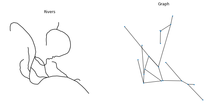
1.3Plot
f, ax = plt.subplots(1, 2, figsize=(12, 6), sharex=True, sharey=True)
rivers.plot(color="k", ax=ax[0])
for i, facet in enumerate(ax):
    facet.set_title(("Rivers", "Graph")[i])
    facet.axis("off")
nx.draw(G, positions, ax=ax[1], node_size=5)
1.4graph to gdf
- nodes:节点gdf
- edges:边gdf
- W:表示节点之间的关系
nodes, edges, W = momepy.nx_to_gdf(G, spatial_weights=True)
nodes.head()
| nodeID | geometry | |
|---|---|---|
| 0 | 0 | POINT (554143.903 9370463.606) |
| 1 | 1 | POINT (558080.528 9366376.590) |
| 2 | 2 | POINT (556297.090 9365917.050) |
| 3 | 3 | POINT (557237.735 9362710.787) |
| 4 | 4 | POINT (556950.010 9367879.530) |
edges.head()
| Length | id | geometry | mm_len | node_start | node_end | |
|---|---|---|---|---|---|---|
| 0 | 8726.582 | 0 | LINESTRING (554143.903 9370463.606, 554090.774... | 8723.436442 | 0 | 1 |
| 1 | 1884.698 | 6 | LINESTRING (558080.528 9366376.590, 557602.861... | 1884.022069 | 1 | 7 |
| 2 | 2233.621 | 8 | LINESTRING (558080.528 9366376.590, 558315.077... | 2232.823547 | 1 | 8 |
| 3 | 2306.128 | 21 | LINESTRING (558080.528 9366376.590, 558150.800... | 2305.303826 | 1 | 8 |
| 4 | 4257.036 | 1 | LINESTRING (556297.090 9365917.050, 555900.606... | 4255.498818 | 2 | 3 |
W.neighbors #键是节点id ,值是邻接边id
{0: [1],
 1: [0, 7, 8],
 2: [3],
 3: [2, 5, 6],
 4: [5],
 5: [3, 4, 7],
 6: [3, 7, 10],
 7: [1, 5, 6],
 8: [1, 9, 10],
 9: [8, 12, 16],
 10: [6, 8, 14],
 11: [12],
 12: [9, 11, 13],
 13: [12],
 14: [10, 15, 17],
 15: [14],
 16: [9],
 17: [14, 18, 19],
 18: [17],
 19: [17]}
W.weights #键是节点ID,值是邻接边权重的list
{0: [1.0],
 1: [1.0, 1.0, 1.0],
 2: [1.0],
 3: [1.0, 1.0, 1.0],
 4: [1.0],
 5: [1.0, 1.0, 1.0],
 6: [1.0, 1.0, 1.0],
 7: [1.0, 1.0, 1.0],
 8: [1.0, 1.0, 1.0],
 9: [1.0, 1.0, 1.0],
 10: [1.0, 1.0, 1.0],
 11: [1.0],
 12: [1.0, 1.0, 1.0],
 13: [1.0],
 14: [1.0, 1.0, 1.0],
 15: [1.0],
 16: [1.0],
 17: [1.0, 1.0, 1.0],
 18: [1.0],
 19: [1.0]}
2.读取街道数据,构造priaml graph
2.1读取momepy中的示例数据
streets = gpd.read_file(momepy.datasets.get_path("bubenec"), layer="streets")
streets.head()  #
| geometry | |
|---|---|
| 0 | LINESTRING (1603585.640 6464428.774, 1603413.2... |
| 1 | LINESTRING (1603268.502 6464060.781, 1603296.8... |
| 2 | LINESTRING (1603607.303 6464181.853, 1603592.8... |
| 3 | LINESTRING (1603678.970 6464477.215, 1603675.6... |
| 4 | LINESTRING (1603537.194 6464558.112, 1603557.6... |
streets.plot() #街道
<AxesSubplot:>

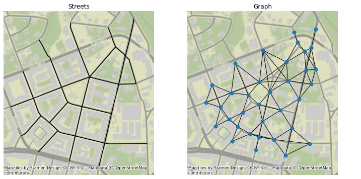
2.2构造primal graph
G_primal = momepy.gdf_to_nx(streets,approach="primal")
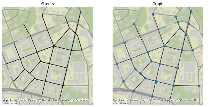
2.3 Plot
f, ax = plt.subplots(1, 2, figsize=(12, 6), sharex=True, sharey=True)
# 初始的街道数据,gdf
streets.plot(color="k", ax=ax[0])
for i, facet in enumerate(ax):
    facet.set_title(("Streets", "Graph")[i])
    facet.axis("off")
    add_basemap(facet)
# graph可视化
nx.draw(
    G_primal, {n: [n[0], n[1]] for n in list(G_primal.nodes)}, ax=ax[1], node_size=50
)
3.构建对偶图
- mommy将行属性存储为节点属性,并自动测量line之间的角度。
G_dual = momepy.gdf_to_nx(streets, approach="dual")
<networkx.classes.multigraph.MultiGraph at 0x280eb0a2e00>
3.1对偶图可视化
# 对偶图可视化
f, ax = plt.subplots(1, 2, figsize=(12, 6), sharex=True, sharey=True)
streets.plot(color="k", ax=ax[0])
for i, facet in enumerate(ax):
    facet.set_title(("Streets", "Graph")[i])
    facet.axis("off")
    add_basemap(facet)
nx.draw(G_dual, {n: [n[0], n[1]] for n in list(G_dual.nodes)}, ax=ax[1], node_size=50)
plt.show()
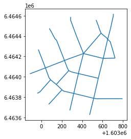
3.2 对偶图to gdf
lines = momepy.nx_to_gdf(G_dual)
lines.head() #对偶图to gdf ,返回原始line的geometry
| geometry | mm_len | |
|---|---|---|
| 0 | LINESTRING (1603585.640 6464428.774, 1603413.2... | 264.103950 |
| 1 | LINESTRING (1603607.303 6464181.853, 1603592.8... | 199.746503 |
| 2 | LINESTRING (1603287.304 6464587.705, 1603286.8... | 382.501950 |
| 3 | LINESTRING (1603363.558 6464031.885, 1603376.5... | 203.014090 |
| 4 | LINESTRING (1603413.206 6464228.730, 1603274.4... | 198.482724 |
# 从下图可以看到,对偶图转为gdf时, 返回原始line的geometry
lines.plot()
<AxesSubplot:>


 2125
2125


 被折叠的 条评论
为什么被折叠?
被折叠的 条评论
为什么被折叠?
 到【灌水乐园】发言


