Coursera自然语言处理专项课程04：Natural Language Processing with Attention Models笔记 Week03（完结）

Natural Language Processing Specialization

Introduction
https://www.coursera.org/specializations/natural-language-processing

Certificate

Natural Language Processing with Attention Models

Course Certificate

本文是学习这门课 Natural Language Processing with Attention Models的学习笔记，如有侵权，请联系删除。

Week 03: Question Answering

Explore transfer learning with state-of-the-art models like T5 and BERT, then build a model that can answer questions.

Learning Objectives

---

• Gain intuition for how transfer learning works in the context of NLP
• Identify two approaches to transfer learning
• Discuss the evolution of language models from CBOW to T5 and Bert
• Fine-tune BERT on a dataset
• Implement context-based question answering with T5
• Interpret the GLUE benchmark

Week 3 Overview

Good to see you again. In this week, you will learn
about transfer learning, which is a new concept
in this course. Transfer learning
allows you to get better results and
speeds up training. You’ll also be looking
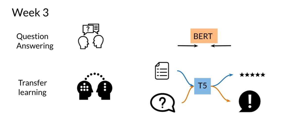
at question answering. Let’s dive in. In Week 3 of Course 4, you’re going to cover many
different applications of NLP. One thing you are going to
look at is question answering. Given the question
and some context, can you tell us what the answer is going to be
inside that context? Another thing you’re going to
cover is transfer learning. For example, knowing some information by training something
in a specific task, how can you make use of that information and apply
it to a different task? You’re going to look at BERT, which is known as the Bidirectional
Encoder Representation which makes use of transformers. You’ll see how you can use bi-directionality to
improve performance. Then you’re going to
look at the T5 model. Basically, what this model
does, you can see here, it has several possible inputs. It could be a question,
you get an answer. It could be a review, and you’ll get the
rating over here. It’s all being fed
into one model.

Let’s look at
question answering. Over here you have context-based
question answering, meaning you take
in a question and the context and it
tells you where the answer is inside
that context over here. This is the highlighted
stuff which is the answer. Then you have closed book question answering
which only takes the question and it returns the answer without having
access to a context, so it comes up with
its own answer. Previously we’ve
seen how innovations in model architecture improve performance and we’ve also seen how data preparation could help. But over here, you’re going
to see that innovations in the way the training is being done also improves performance. In which case, you will see how transfer learning will
improve performance. This is the classical training that you’re used to seeing. You have a course review, this goes through a model, and let’s say you
predict the rating. Then you just predict
the rating the same way as you’ve
always been doing. Nothing changed here, this is just an overview of the classical training
that you’re used to.

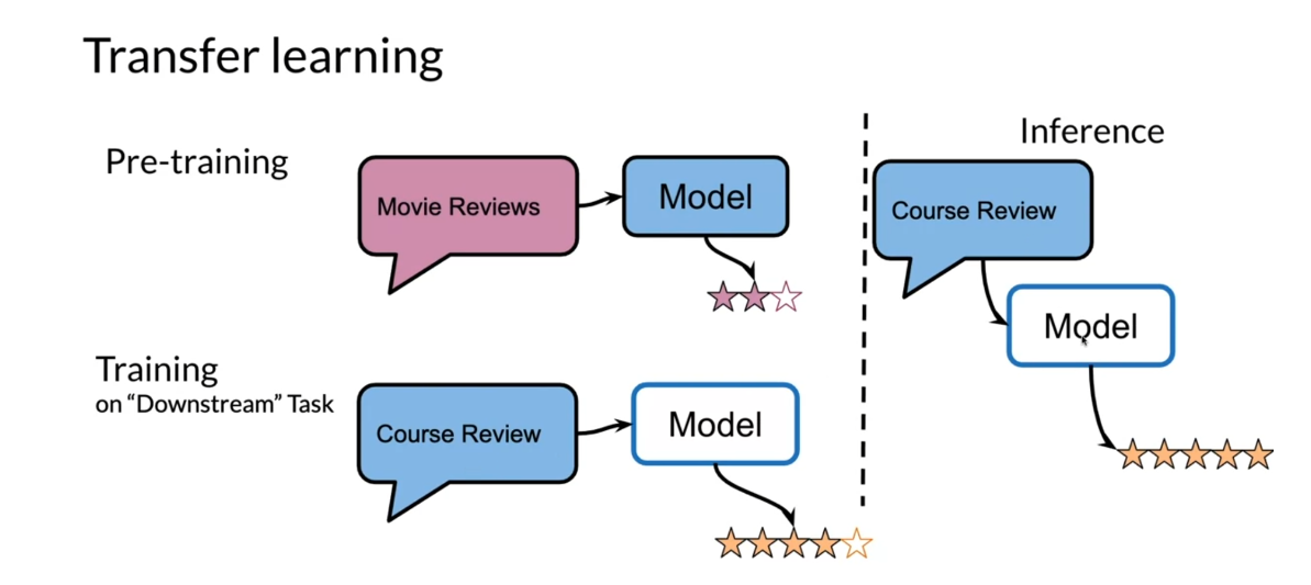
Now, in transfer learning, let’s look at this example. Let’s say that you
have movie reviews and then you feed them into your model and you
predict a rating. Over here you have
the pre-train task, which is on movie reviews. Now, in training, you’re going to take the existing model
for movie reviews, and then you’re going to find two units or train it again, on course reviews, and you’ll predict the
rating for that review. As you can see over here, instead of initializing
the weights from scratch, you start with the
weights that you got from the movie reviews, and you use them as the starter points when training
for the course reviews. At the end, you do some
inference over here, and you do the inference the same way you’re used to doing. You just take the course review, you feed this into your model, and you get your prediction.

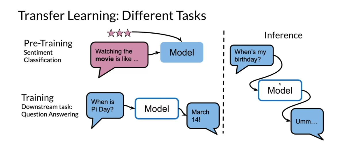
You can also use transfer
learning on different tasks. This is another
example where you feed in the ratings
and some review, and this gives you
sentiment classification. Then you can train it on a downstream task like
question answering, where you take the
initial weights over here and you train it on question
answering. When is Pi day. The model answers March 14th. Then you can ask them
model the same question. When’s my birthday over here? It does not know the answer. But this is just
another example of how you can use transfer
learning on different tasks.

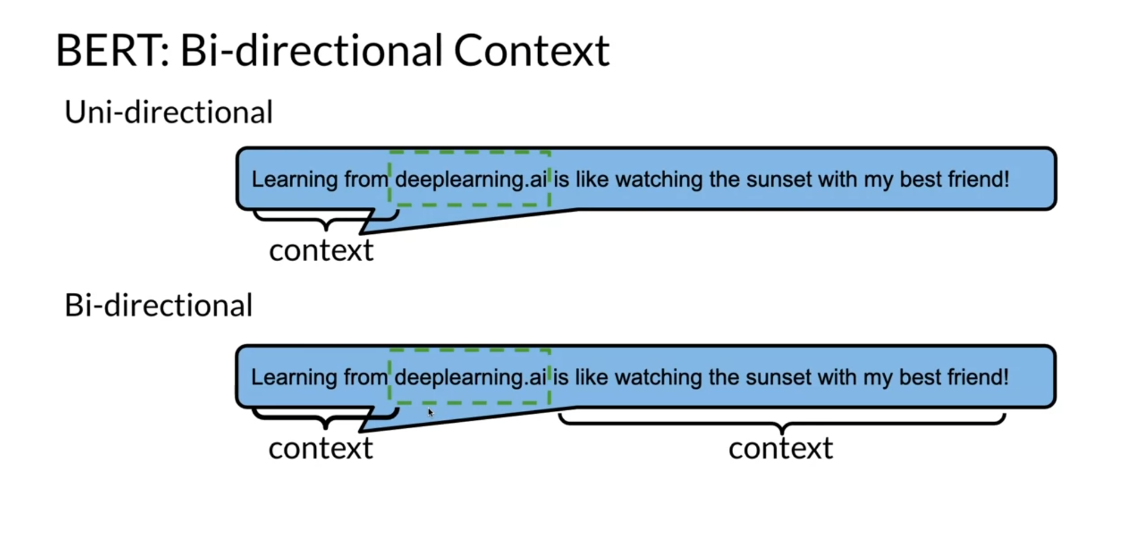
Now we’re going to look at BERT, which makes use of
bi-directional context. In this case, you have
learning from deeplearning.ai, is like watching the sunset
with my best friend. Over here the context is
everything that comes before. Then let’s say you’re
trying to predict the next word, deeplearning.ai. Now, when doing bi-directional
representations, you’ll be looking at the
context from this side and from this side to
predict the middle word. This is one of the main
takeaways for bi-directionality.

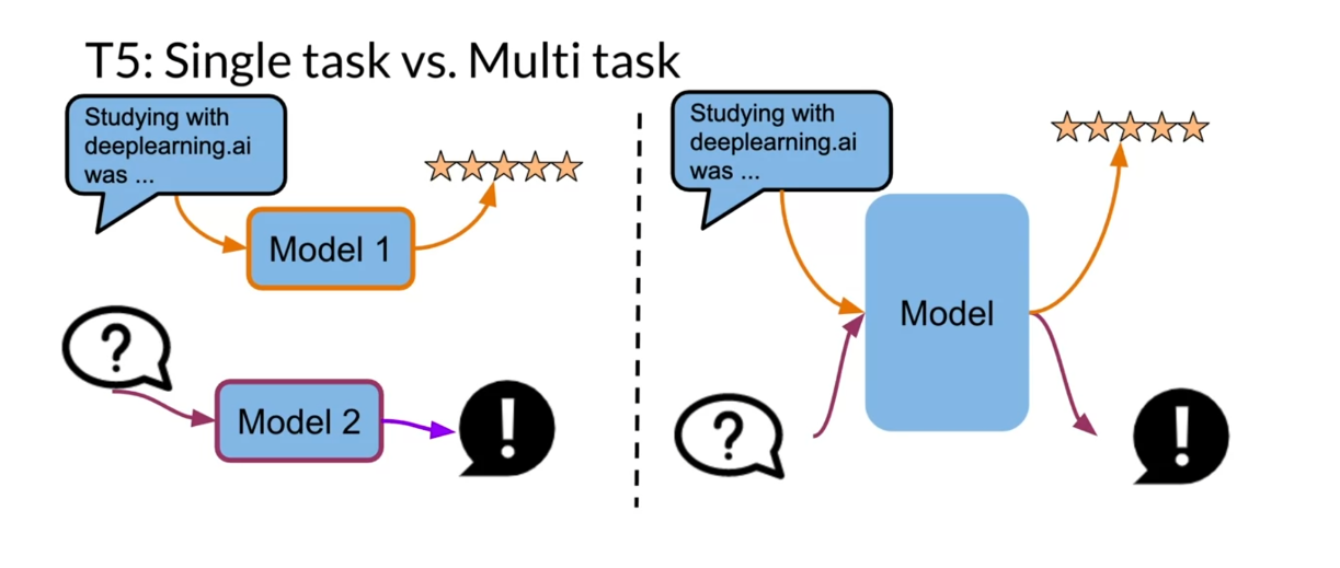
Now let’s look at single
task versus multitask. Over here you have a single
model which takes in a review and then
predicts a rating. Over here you have
another model which takes in a question and
predicts an answer. This is a single task each, like one model per task. Now, what you can
do here with T5 is, it is the same
model that’s being used to take the review, predict the rating, and
then take the question, and predict the answer. Instead of having two
independent models, you end up having one model.

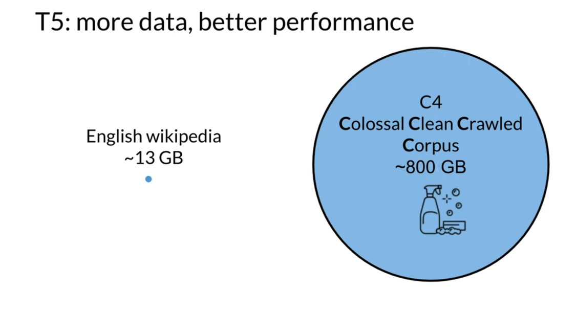
Let’s look at T5. Over here, the main takeaway is that the more data you have, generally the better
performance there is. For example, the English
Wikipedia dataset is around 13 gigabytes
compared to the C4, Colossal Clean Crawled Corpus
is about 800 gigabytes, which is what T5 was trained on. This is just to
give you like how much larger the C4 dataset is, when compared to the
English Wikipedia.

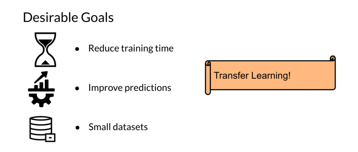
What are the desirable goals
for transfer learning? First of all, you want to reduce training time because you already had a pre-trained model. Hopefully, once you
use transfer learning, you’ll get faster convergence. It will also improve
predictions because you’ll learn a few things from
different tasks that might be helpful and useful for your currents predictions on
the task you’re training on. Finally, you might
require or need less data because your model
has already learned a lot from other tasks. If you have a smaller dataset, then transfer learning
might help you. You now know what
you’re about to learn. I’m very excited to show
you all these new concepts. In the next video, we’ll start by exploring
transfer learning.

Transfer Learning in NLP

This week, I’ll be talking about transfer learning with
the full transformer. I’ll also talk a
little bit about BERT, which is the Bidirectional
Encoder Representation for Transformers. Then I’ll talk about a special model known
as the T5 model, what you learned about. Now all of these concepts make
use of transfer learning. What is transfer learning?
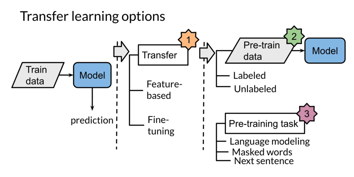
Let me show you. You’ll now take a look at the
transfer learning options that you will have while
performing your NLP tasks. This is a quick recap where
you have your train data, goes into a model, then you have a prediction. Transfer learning will
come in two basic forms. The first one is using
feature-based learning, and the other one is
using fine-tuning. By feature-based, I mean things like word
vectors being learnt. Fine-tuning is you take an existing model,
existing weights, and then you tweak them a
little bit to make sure that they work on the specific
task you’re working on. There is pre-trained
data which makes use of labeled and
unlabeled data, let’s say you’re training your model on sentiments
for product reviews. Then you can use those
same weights to train your model on course reviews. Then the other thing
is pre-training task, which usually makes use
of language modeling. For example, you mask a word and you try to
predict what that word is, or you try to predict what
the next sentence would be.

Let’s look at
general-purpose learning, and this is something that
you’re already familiar with. Over here you have
I am because I’m learning and you’re trying
to predict the central word. The central word is
happy over here. You used a model known as the continuous
bag-of-words model. Or at least you got the
following embeddings. Now you can use
these embeddings as the inputs features and translation tasks to translate
from English to German.

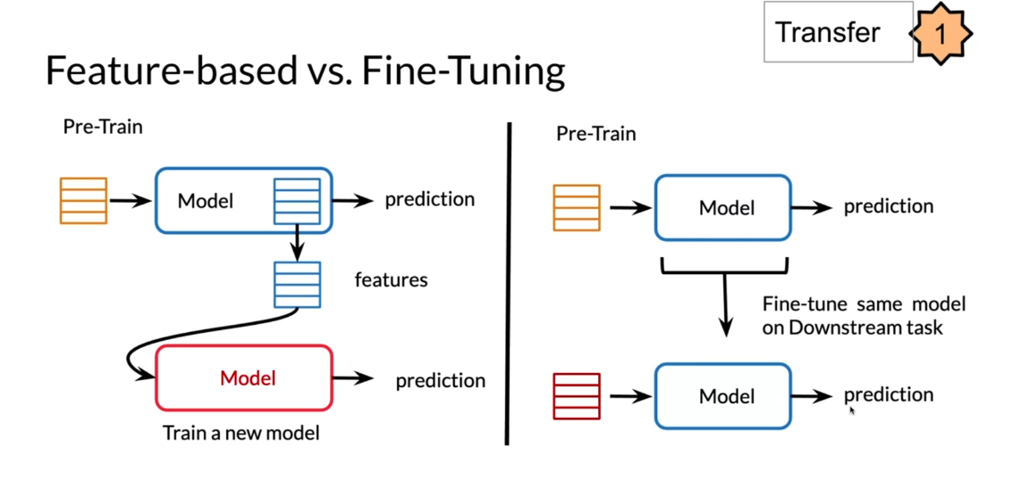
Let’s look at a more
concrete example of feature-based
versus fine-tuning. Where you have word embeddings, put it in your model, you get a prediction. Then over here you get some type of new features
or new word embeddings. Then you feed them into a
completely different model. This gives you your prediction. Now, on the fine-tuning side, you have your embeddings, you feed it into your model, you get a prediction, and then you fine-tune
on this model, on the downstream task. Then you have some new inputs
on your new weight so that you fine-tune so you feed it
in and you get a prediction.

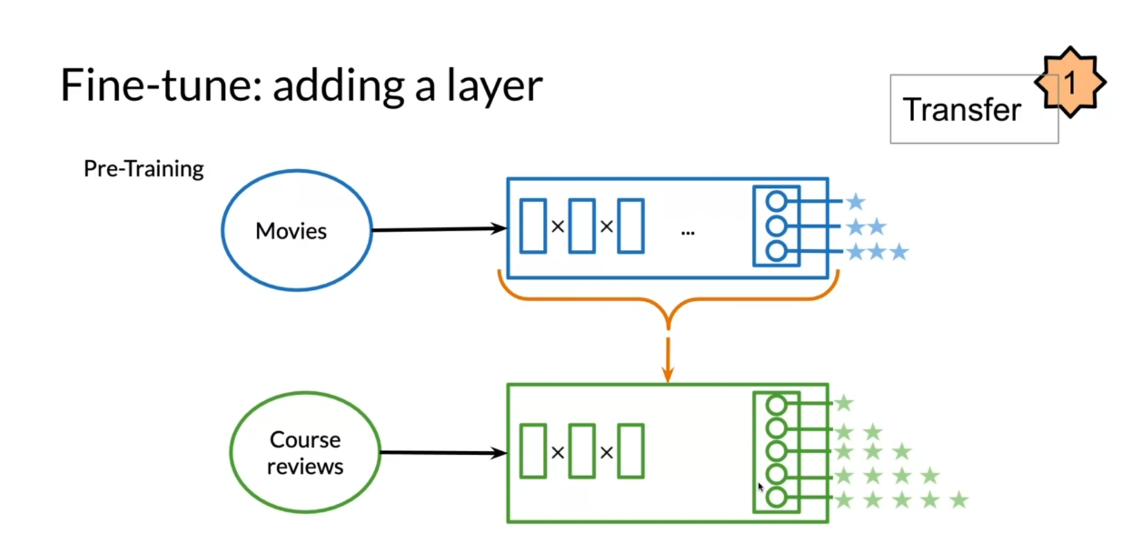
Let’s look at fine-tuning. This is a way to add
fine-tuning to your model. Let’s say you have movies and
you’re predicting one star, two stars, or three stars. You pre-trained and let’s say now you have course reviews. One way you can do this is you fix all of these weights
that you already have. Then you add a new
feed-forward network while keeping everything
else frozen here. Then you just tune on this new network
that you just added.

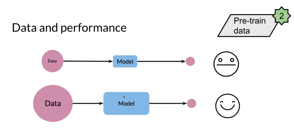
Data affects performance a lot. In this case, you have
data being fed into your model and you get
some neutral outcome. But as you have more data and you build a larger
model over here, then you get a much
better outcome. The more data you have, the better it is, and
the more data you have, the bigger the models
you can build will be able to capture the task
you’re trying to predict on.

Let’s look at labeled
versus unlabeled data. Now, this is just
a graphic example that tells you that usually you’ll have way more
unlabeled text data than labeled text data. Here’s an example. In pre-training you
have no labels. You feed this into your model. Then in downstream task, you could have something like, what day is Pi day, feed this into your model
and you get the March 14th. Remember, these are the word vectors we’re talking about.

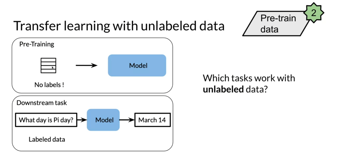
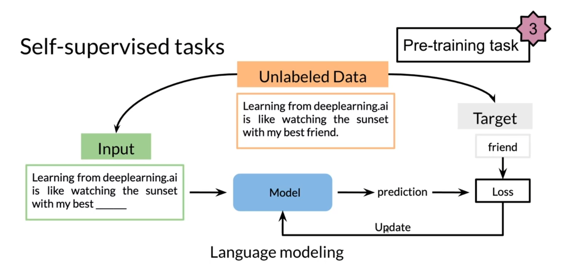
Which tasks work
with unlabeled data? This is a self-supervised task, so you have the unlabeled data, and then you create
input features. You create targets or labels. This is how it works. You have unlabeled data, learning from
deep-learning AI is like watching the sunset
with my best friend. You create the inputs
and then blank. The sunset with my best blank. You’re trying to predict friend. You feed this into your model. You get your prediction. The target is friend, here prediction goes in. You have the loss
here and then you use this loss to
update your model. This is basic language modeling that you’ve already seen before.

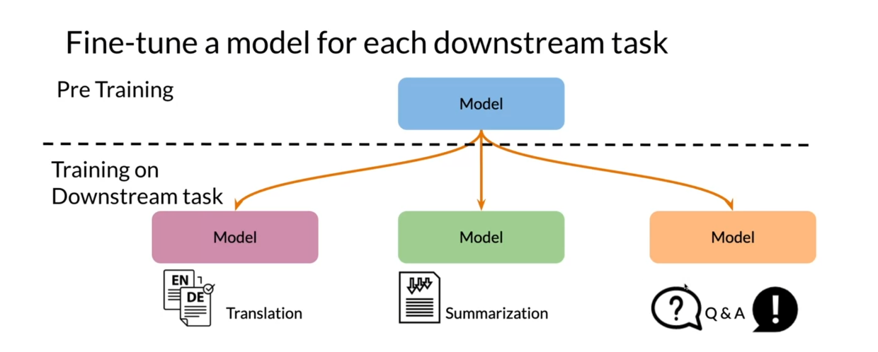
Let’s look at fine-tuning a
model in the downstream task. You have your model here. You did some pre-training
on it either by masking words or predicting
the next sentence. Then use this model to train
it on downstream tasks. You can use this model, fine-tune it on translation or summarization, or
question answering.

Here’s a summary of what
you’ve seen so far. Usually you have
some train data, you have the model,
you make a prediction. We use transfer learning to get feature-based examples
or fine-tuning. Feature-based like word
vectors or word embeddings and fine-tuning is something that’s you can do on downstream tasks. Then we can also use labeled data and unlabeled
data to help us. You can train something on a different task on a
different data set. and that will also
help a little bit. Then you can use
pre-training task like language modeling
or masked words or next sentence prediction. You have now seen some
advantages of transfer learning.

ELMo, GPT, BERT, T5

I’ll show you a
chronological order of when the models
were discovered. We will also see the advantages and the disadvantages
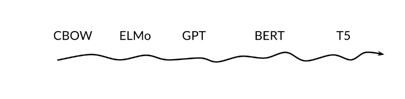
of each model. Let’s start. This is a quick outline where you can see we start here with
continuous bag of words model, then we got ELMo, then we got GPT, then we got BERT AND finally we ended up having
T5 and so more. Like over here we’re
going to end up having many more models coming
up, hopefully soon. This is not a
complete history of all relevant models
and research findings, but it’s useful to see
what problems arise with each model and what
problems each model solves. Let’s look at context over here. Let’s say we have
the word right. Ideally, we want to see
what this word means. We can look at the
context before it. Then we can also look at
the context after it. That’s how we’ve been able to train word
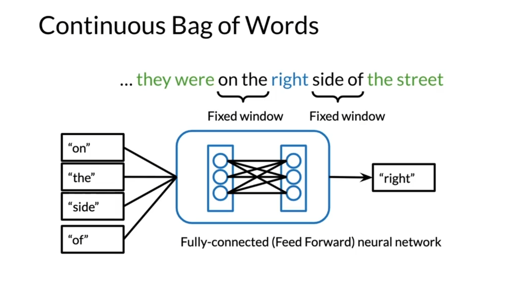
embeddings so far. The continuous bag
of words over here, you have the word right. Previously what
you’ve been doing, you would take a fixed window, say two before and two
after, or three or four, whatever as CS is
for the window size. Then you’ll take the
corresponding words, feed them into a neural network, and predict the central word in this case, which is right. Now the issue over here is that, what if we wanted to look at
not only the fixed window, but all the words before
and all the words after.

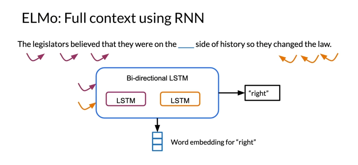
How can we do that? If
you want more context. They were on D over here. This is the first left part of the sentence and then all the right parts
of the sentence. Instead of having
the fixed window, we want to add the streets
or history for example. To use all of the context words, what researchers have done, they explored the
following using RNN. They would use an RNN from
the right and from the left. Then they would have a
bi-directional LSTM, which is a version of
recurrent neural network. You feed both of them in. Then you can predict
the center word right. That gives you the word
embedding for the word, right.

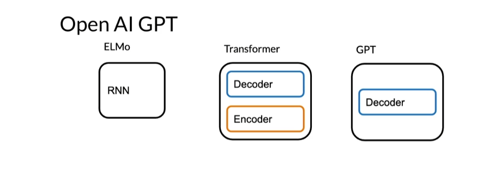
Now, open AI GPT what it did. We had transformer, the encoder decoder architecture that
you’re familiar with. Then we ended up having
this GPT which makes use of a decoder of stacks only. In this case we only
have one decoder, but you can have several
decoders in the picture. ELMo made use of RNNs or LSTMs. We would use these models to
predict the central word.

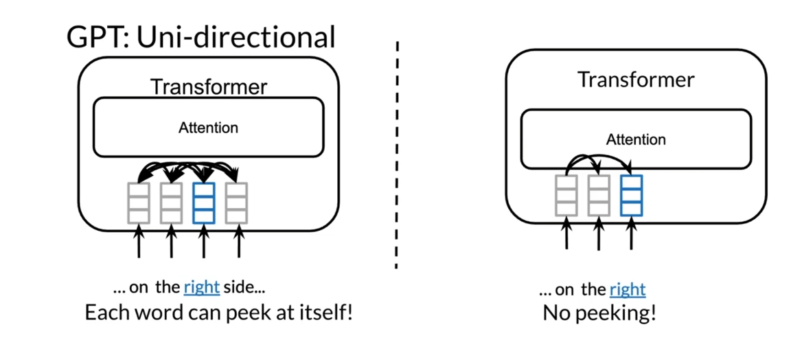
Why not use a
bi-directional model? In this case, this
is the transformer, and you can see that in
the transformer over here, each word can peek at itself. If we were to use it for under, right, you can only
look at itself. But the issue is that
you cannot peek forward. Remember, you’ve seen
this in causal attention where you don’t look
forward you only look at the previous ones.

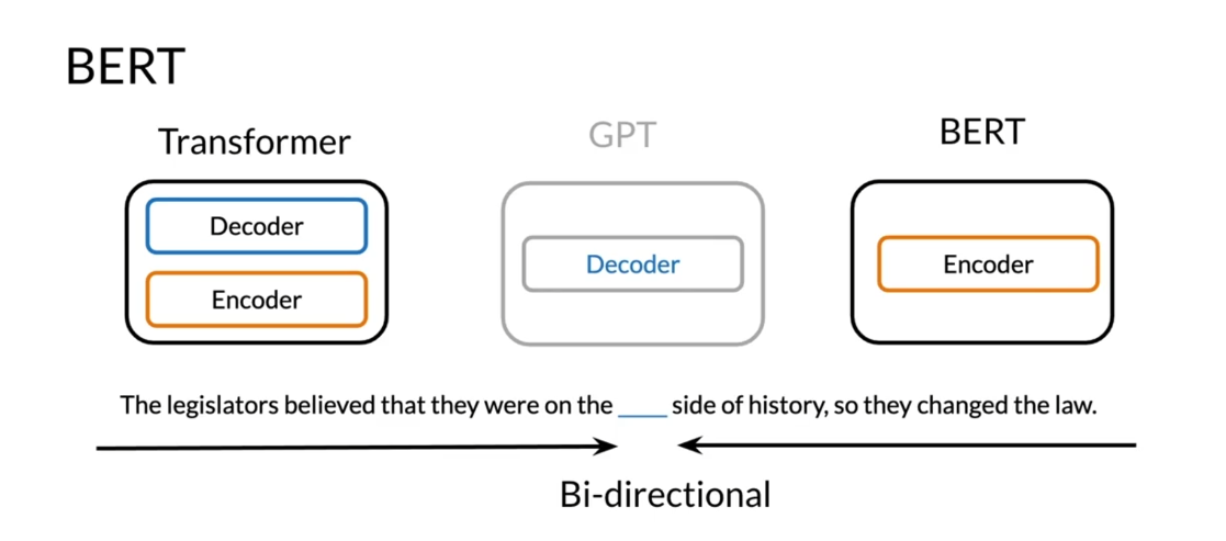
BERT came and helped
us solve this problem. This is a recap. Transformers, encoder decoder, GPT makes use of decoders and BERTs makes use of encoders. Over here you have
the Legislature believed that they were on
the blank side of history, so they changed the law. Over here we can make use of bi-directional encoder
representations from transformers and this will
help us solve this issue.

This is an example
of a transformer plus bi-directional context. You feed this into your model and then you get right and of. Because of this,
you’re able to look at the sentence from
the beginning and from the end and make use of the context to predict
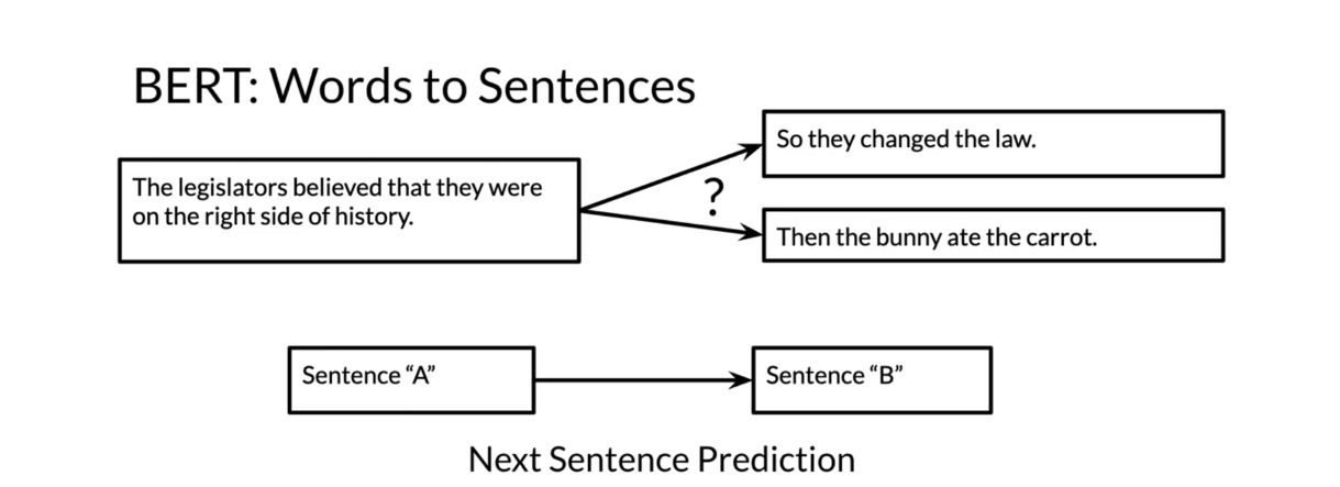
the corresponding words. If we’re to look at
words to sentences, meaning instead of trying
to predict just the word, we’ll try to predict what
the next sentence is. Given the sentence over here, the legislators believed that they were on the right
side of history. Is this the next sentence or
is this the next sentence? You have a sentence A and then you try to predict
the next sentence B. In this case it’s obviously
so they changed the law.

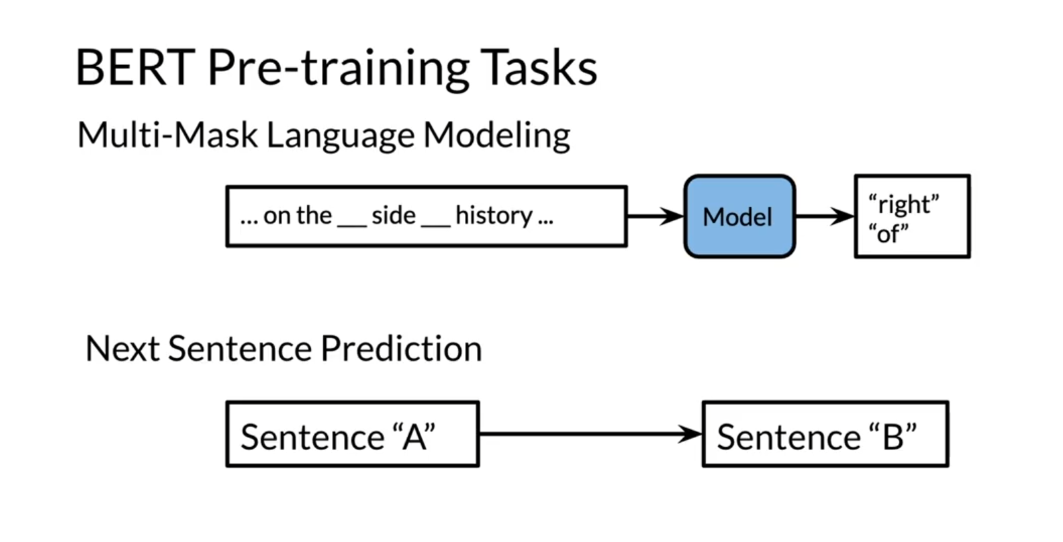
BERT pre-training tasks makes use of multi-mask
language modeling. The same thing that
you’ve seen before and it makes use of the next
sentence prediction. It takes two sentences
and it predicts whether it’s a yes
meaning sentence two follow sentence one, or sentence B follow
sentence A or not.

BERT（Bidirectional Encoder Representations from Transformers）预训练模型在预训练过程中使用了两种任务：

1. 掩码语言建模（Masked Language Modeling，MLM）：在这个任务中，BERT会随机地将输入序列中的一些单词标记为 [MASK]，然后尝试根据上下文预测这些被掩码的单词。这个任务可以让模型学习到单词之间的语义关系和上下文信息。

2. 下一句预测（Next Sentence Prediction，NSP）：在这个任务中，BERT会接收一对句子作为输入，然后预测第二个句子是否是第一个句子的下一个句子。这个任务可以帮助模型学习到句子之间的逻辑关系和连贯性。

通过这两种任务的预训练，BERT模型可以学习到丰富的语言表示，从而在下游任务中取得良好的效果，例如问答、文本分类和命名实体识别等任务。

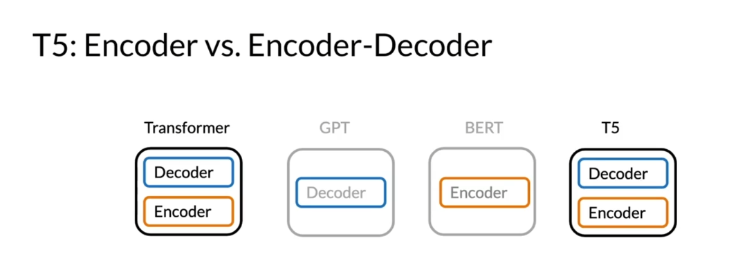
Let’s look at encoder
versus encoder decoder. Over here you have
the transformer, which had the encoder
and the decoder stack. Then you had GPT, which just had decoder stack, and then BERT, just
the encoder stack. T5 tested the
performance when using the encoder decoder as in the
original transformer model. The researchers
found that the model performed better when it contained both the encoder
and the decoder stacks.

Let’s look at the multi-task
training strategy over here so you have studying
with deeplearning.ai was. It’s being fed into the model and it gives you a
five star rating. Hopefully it’s a
five star rating. Then you have a question and
then you get the answer. But the question here is, how do you make sure that the model knows which
task it’s performing in? Because you can feed
in a review over here. How do you know
that it’s not going to return an answer instead? How do you know it’s
going to return a rating? Or if you feed in a question, how do you know it’s
not going to return some numerical outputs or some text version of
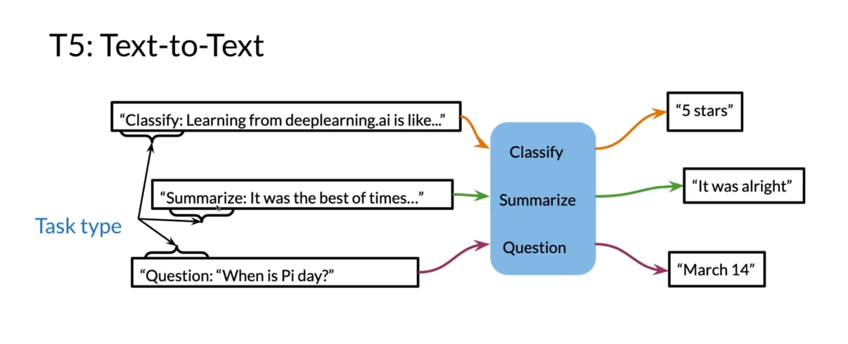
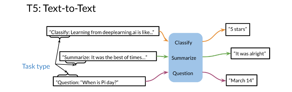
a numerical output? Let’s see how to do this. Over
here is an example where, let’s say you’re trying
to classify whether this is five stars or four
stars or three stars. You append the string,
classify for example. Then it classifies it
and you get five stars. Let’s say you want to summarize, so you add the string
summarize colon. It goes into the model. It’s automatically identifies
that you’re trying to summarize and it says
that it was all right. You have a question you
append question string. It knows that it’s a question
and it returns the answer. Now, this might not be the exact text that
you’ll find in the paper, but it gives you the
overall sense of the idea.

T5（Text-to-Text Transfer Transformer）是一种基于Transformer架构的通用文本生成模型，其预训练任务是文本到文本的转换。具体来说，T5的预训练任务是将输入文本转换为目标文本，可以是生成式任务（如翻译、摘要生成等）或分类任务（如文本分类、命名实体识别等）。

T5的预训练过程包括以下步骤：

1. 输入-输出对构建：从大规模文本数据中构建输入-输出对，即将输入文本和目标文本组成的文本对。这些文本对可以是原始文本和重写文本、问题和答案等。

2. 文本转换模型：使用Transformer架构构建文本转换模型，该模型由编码器和解码器组成。编码器将输入文本编码为上下文表示，解码器使用这些表示生成目标文本。

3. 预训练任务：使用文本对作为输入-输出对，通过最大似然估计（MLE）或其他适当的损失函数来训练模型。模型的目标是最大化生成目标文本的概率。

T5的设计使其适用于各种文本生成任务，通过微调预训练模型，可以在特定的下游任务上取得良好的性能。

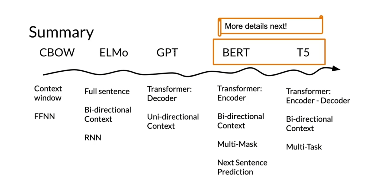
In summary, you’ve seen the continuous bag
of words model, which makes use of a
fixed context window. You’ve seen ELMo, which makes use of a
bi-directional LSTM. You’ve seen GPT, which
is just a decoder stack, and you can see
uni-directional in context. Then you’ve seen BERT, which makes use of bi-directional encoder
representation from the transformer, and it also makes use of multi-mask language modeling and next sentence prediction. Then you’ve seen the
T5 which makes use of the encode decoder
stack and also makes use of mask and
multi-task training. You have now seen an
overview of the models. You have seen how the text
to text model has a prefix. With the same model, you
can solve several tasks. In the next video, we will be looking at the birth
model in more detail, also known as the Bidirectional Encoder representation
for Transformers.

Reading: ELMo, GPT, BERT, T5

The models mentioned in the previous video were discovered in the following order.

In CBOW, you want to encode a word as a vector. To do this we used the context before the word and the context after the word and we use that model to learn and create features for the word. CBOW however uses a fixed window C (for the context).

What ElMo does is, it uses a bi-directional LSTM, which is another version of an RNN and you have the inputs from the left and the right.

Then Open AI introduced GPT, which is a uni-directional model that uses transformers. Although ElMo was bi-directional, it suffered from some issues such as capturing longer-term dependencies, which transformers tackle much better.

After that, the Bi-directional Encoder Representation from Transformers (BERT) was introduced which takes advantage of bi-directional transformers as the name suggests.

Last but not least, T5 was introduced which makes use of transfer learning and uses the same model to predict on many tasks. Here is an illustration of how it works.

Bidirectional Encoder Representations from Transformers (BERT)

I’ll now teach you about Bidirectional Encoder
Representations for Transformers, or in short, just BERT. BERT is a model that makes
use of the transformer, but it looks at the inputs
from two directions. Let’s dive in and
see how this works. Today, you’re going
to learn about the BERT architecture
and then you’re going to understand how BERT
pre-training works and see what the inputs
are and the outputs are. What is BERT? BERT is the Bidirectional
Encoder representations from transformers, and it makes use of transfer
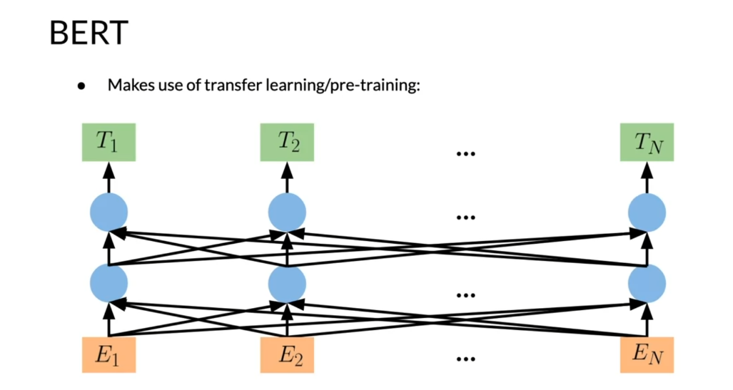
learning and pre-training. How does this work?
Usually starts with some inputs embeddings, so E_1, E_2, all the way to some
random number E_n. Then you go through some transformer blocks,
as you can see here. Each blue circle is
a transformer block, goes up furthermore and then you get your T_1, T_2, T_n. Basically, there
are two steps in BERT’s framework,
pre-training and fine-tuning. During pre-training,
the model is trained on unlabeled data over different
pre-training tasks, as you’ve already seen before. For fine tuning,
the BERT model is first initialized with a
pre-trained parameters, and all of the parameters
are fine-tuned using labeled data from
the downstream tasks. For example in the
figure over here, you get the corresponding
embeddings, you run this through a
few transformer blocks and then you make
the prediction.

We’ll discuss some
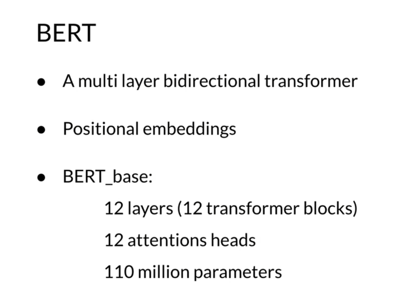
notation over here. First of all, BERT a multi-layer
bidirectional transformer. It makes use of
positional embeddings. The famous model is BERT’s base, which has 12 layers or
12 transformer blocks, 12 attention heads, and
110 million parameters. These new models that are coming out now like GPT-3 and so forth, they have way more
parameters and way more blocks and layers.

Let’s talk about pre-training. Before feeding the word
sequences to the BERT model, we mask 15 percent of the words. Then the training data generator chooses 15 percent of these positions at
random for prediction. Then FDI token is chosen, we replace the ith token with, one, the mask token, 80 percent of the time, and then, two, a random token 10 percent
of the time, and then, three, the unchanged with either token 10
percent of the time. In this case then Ti, what you’ve seen in
the previous slide, will be used to
predict the original token with cross entropy loss. In this case, this is known
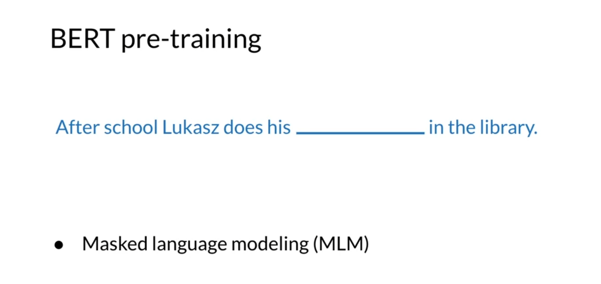
as the masked language model. Over here we have,"
After school, Lucas does his blank in the
library," so maybe work, maybe homework one
of these words that your BERT model is
going to try to predict. To do so usually what you do, you just add a dense layer after the Ti token and use it to classify after the
encoder outputs. You just multiply
the outputs vectors by the embedding
matrix and then to transform them into a
vocabulary dimension and you add a
softmax at the end.

This is another
sentence, “After school, Lucas does his homework in
the library,” and then, “After school blank his
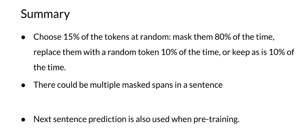
homework in the blank.” You have to predict Lucas does, and then library also. In summary, you choose 15 percent of the
tokens at random. You mask them 80
percent of the time, replace them with a random
token 10 percent of the time, or keep as is 10
percent of the time. Then notice that there could be multiple masked
spans in a sentence. You could mask several
words in the same sentence. In BERT, also next sentence prediction is
also used when pre-training. Given two sentences,
if it’s true, it’s means the two sentences
follow one another. Otherwise, they’re different, they don’t lie in the same
sequence of the text. You have now developed an
intuition for this model. You’ve seen that
BERT makes use of the next sentence prediction and masked language modeling. This allows the model to have a general sense of the language. In the next video, I’m going to formalize this and show you the loss
function for BERT. Please go onto the next video.

BERT Objective

I will be talking about
the BERT objective. You’ll see what you are
trying to minimize. Specifically, I’ll show you how you can combine
word embeddings, sentence embeddings, and
positional embeddings as inputs. Let’s take a look at
how you can do this. You’re going to learn how
BERT inputs are fed into the model and the
different types of inputs and their structures. Then you’re going to visualize
the output and finally, you’re going to learn
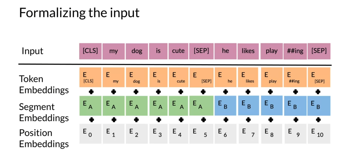
about the BERT objective. Formalizing the input, this is the BERT
input representation. You start with
position embeddings. They allow you to indicate
the position in the sentence of the word where each word is in the corresponding
sentence. So you have this. Then you have the
segment embeddings. They allow you to indicate
whether it’s a sentence A or sentence B because remember in BERT you also use next
sentence prediction. Then you have the
token embeddings or the input embeddings. You also have a CLS token, which is used to indicate the
beginning of the sentence, and a SEP token, which is used to indicate
the end of the sentence. Then what you do, you just take the sum of the
token embeddings, the segmentation embeddings, and the position embeddings, and then you get your new input.

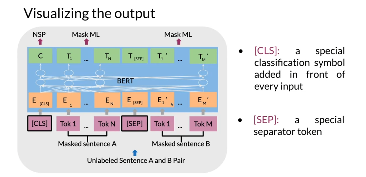
Over here you can see you
have masked sentence A, you have masked sentence B, they go into tokens, and then you have the CLS token, which is a special
classification symbol added in front of every input. Then you have the SEP token, which is the special
separator token. You convert them into
the embeddings so then you get your
transformer blocks. Then you can see at the end
you get your T_1 to T_N, your T_1 prime to T_M prime. Each T_I embedding
will be used to predict the masked word
via a simple softmax. You have this C also, embedding, which can be used for next
sentence prediction.

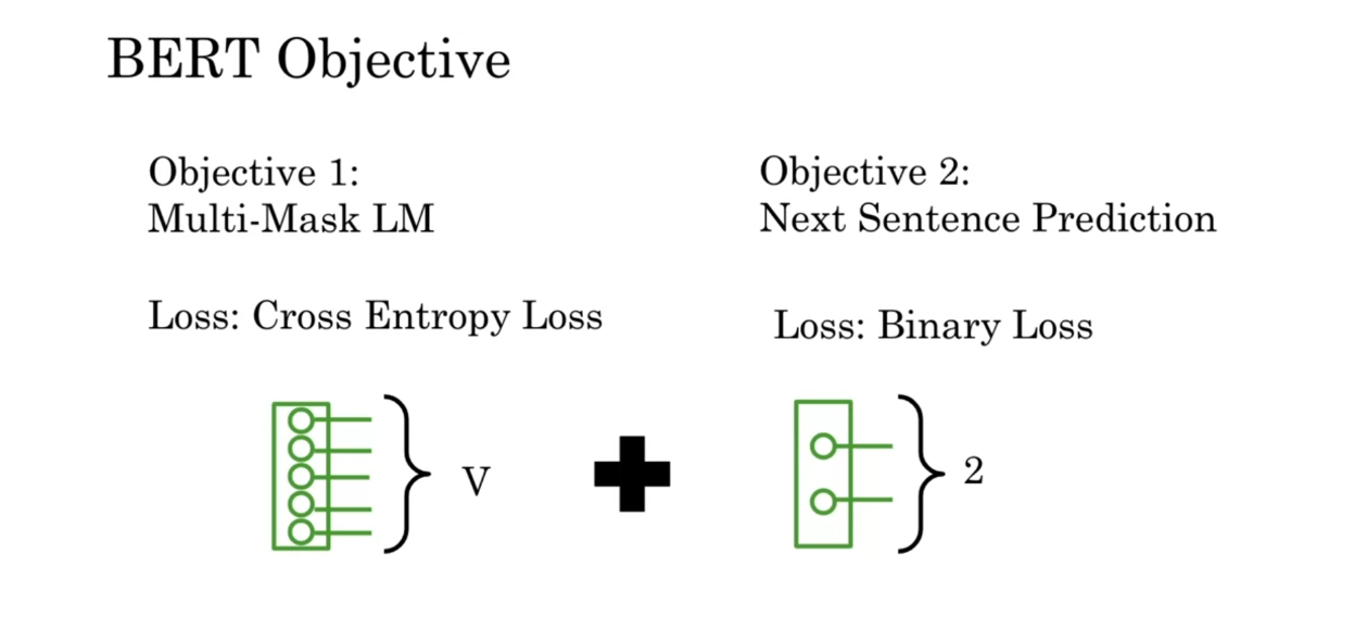
Let’s look at the
BERT objective now. For the Multi-Mask
language model, you use a cross-entropy
loss to predict the word that’s being masked or the
words that are being masked, and then you add this
to a binary loss for the next sentence
prediction so given the two sentences do they
follow one another or not?

In summary, you’ve seen
the BERT objective and you’ve seen the model
inputs and outputs. In the next video, I will show you how you can fine-tune this
pre-trained model. Specifically, I’ll show
you how you can use it to your own tasks
for your own projects. Please go on to the next video.

Reading: BERT Objective

We will first start by visualizing the input.

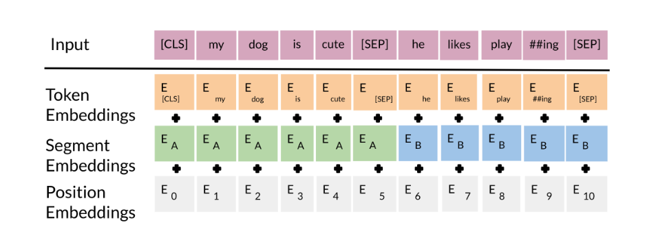
The input embeddings are the sum of the token embeddings, the segmentation embeddings and the position embeddings.

The input embeddings: you have a CLS token to indicate the beginning of the sentence and a sep to indicate the end of the sentence

The segment embeddings: allows you to indicate whether it is sentence a or b.

Positional embeddings: allows you to indicate the word’s position in the sentence.

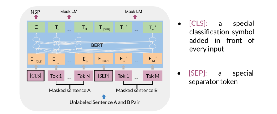
The C token in the image above could be used for classification purposes. The unlabeled sentence A/B pair will depend on what you are trying to predict, it could range from question answering to sentiment. (in which case the second sentence could be just empty). The BERT objective is defined as follows:

You just combine the losses!

If you are interested in digging deeper into this topic, we recommend you to look at this article.

Fine tuning BERT

Using BERT can get you state of the art
results on many tasks or problems. In this video, I’m going to show you
how you can fine tune this model so that you can get it to work
on your own data sets. Let’s take a look at how you can do this. So right now you’re going to
see how you fine tune BERT. So during pre training remember you
had sentence A and sentence B, and then you use next sentence prediction and use the mask tokens to predict the mask
tokens that you mask from each sentence. So that’s in pre training. Now if you want to go on to MNLI or
like hypothesis premise scenario, then instead of having sentence A and
sentence B, you’re going to feed in the hypothesis
over here, and the premise over here. For NER you going to feed in
the sentence A over here, and then the corresponding tags over here. For question answering,
you will have SQuAD, for example, you’ll have your question over here and
then your answer over here.

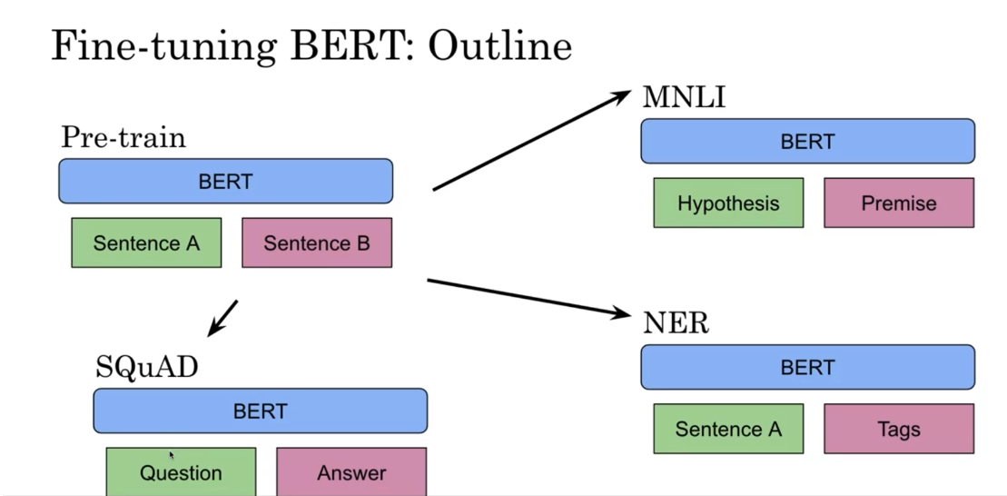
So visually what does this look like? So remember this image
from the BERT paper. So this is what ends up happening. Over here you have the question,
over here you’ll have the paragraph and this will give you like your answer,
that starts in the end for the answer. Then for NER again,
you’ll have the sentence and the correspondent named entities. For MNLI you’ll have the hypothesis and
then the premise and so forth.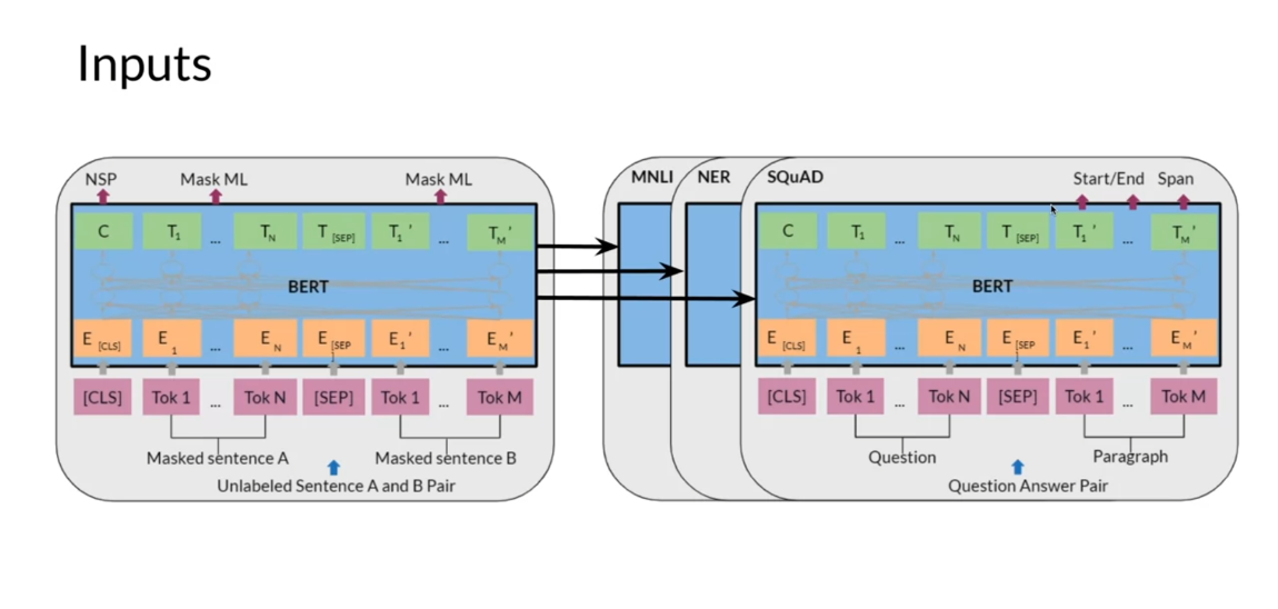

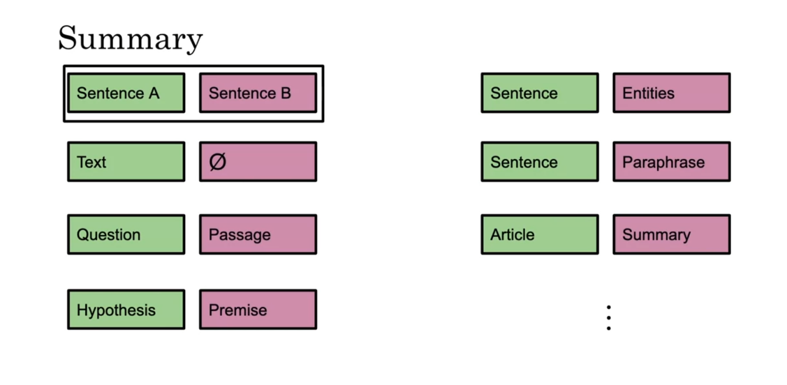
So in summary, given the place
of sentence A and sentence B, you can fill it with a text
in parts four sentence A, and then say like a no symbol to say
that you’re trying to classify the text whether it’s for
sentiment analysis, like happy or sad. So that’s the only way to do it. Question passage for question answering. You could have hypothesis premise for
MNLI. You could have sentence with
the named entities for NER, you can have sentence and
a paraphrase of the sentence. You could have an article in
the summary and so forth. So this is just the inputs
into your BERT model. Now that you know how to fine tune
your model on classification tasks, question answering, summarization and
many more things, we’ll take it to the next level and introduce you
to a new model known as the T5. Please go onto the next video
to learn about the T5 model.

Transformer: T5

The T5 model could be used
on several NLP tasks and it also uses similar
training strategy to birds. Concretely, it makes use of transfer
learning and masked language modeling. The T5 model also uses
transformers when training. So let’s take a look at how you can use
this model in your own applications. >> So you’re going to understand how T5
works, then you’re going to recognize the different types of attention used and
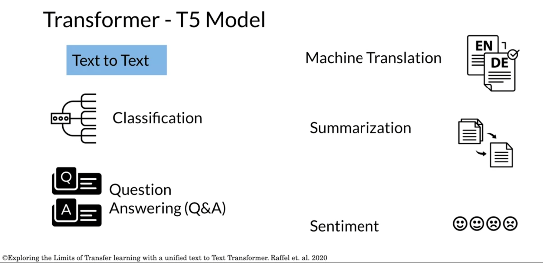
see an overview of the model architecture. So T5 transformers known as
the text to text transformer and you can use it in classification,
you can use it for question answering to answer a question. You can use it for machine translation,
you can use it for summarization and you can use it for sentiments. And there are other applications
that you can use T5 for, but we’ll focus on this for now.

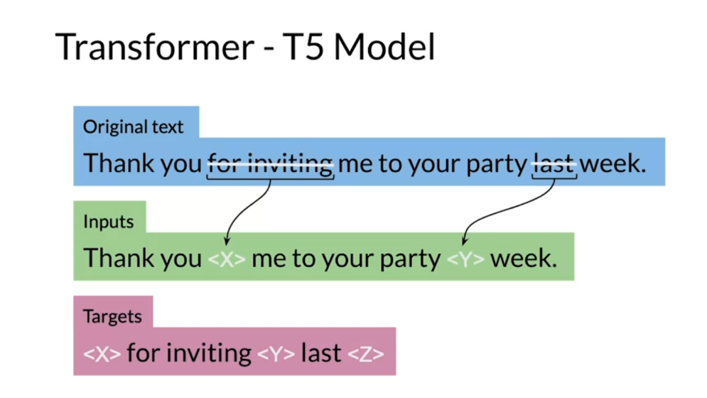
So the model architecture and the way the
pre training is done first of all is you have an original text, something like
this where you have thank you for inviting me to your party last week. So you mask the certain words,
so for inviting me last and then you replace it with these
tokens like brackets X, brackets Y. So brackets X corresponding to for
inviting and brackets why corresponding to last. And your targets are going to be
brackets X for inviting brackets Y last. And these tokens or these brackets like
they keep going in increments order, so then it’s bracket Z, then maybe
brackets A brackets B and so forth.

So each brackets corresponds to a certain
targets, the model architecture and a different transformer architectural
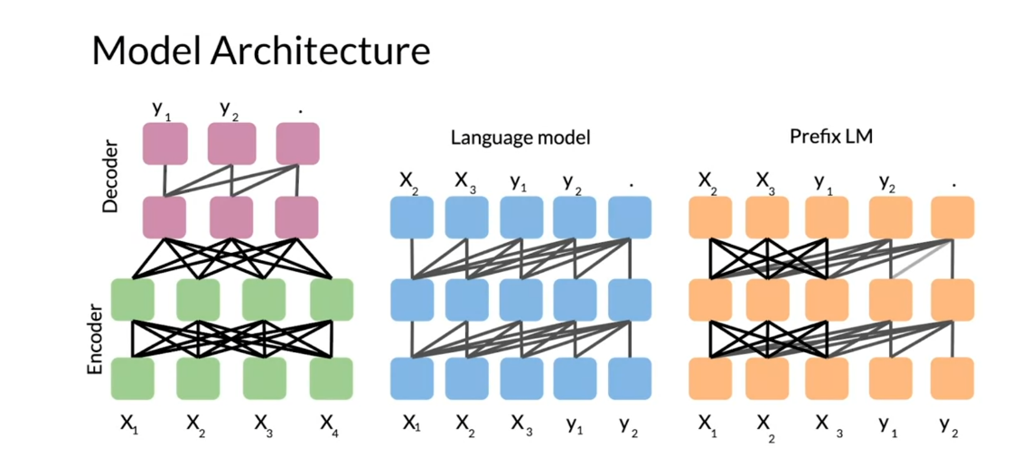
variants that we’re going to consider for the attention party are. So we start with the basic
encoder decoder representation. So you can see over here you have fully
visible attention in the encoder and then causal attention in the decoder and then you have the general encoder decoder
representation just as a notation. So light gray lines correspond
to causal masking and dark gray lines correspond to
the fully visible masking. So on the left, as I said again,
it’s the standard encoder decoder architecture in the middle over here
what we have we have the language model which consists of a single
transformer layers stack and it’s being fed the concatenation
of the input and the target. So it uses causal masking throughout
as you can see because they’re all great lines and you have X1
going inside over here, get a X2. X two goes into the model X three and
so forth. Now over here to the right we
have prefix language model which corresponds to allowing fully visible
masking over the inputs as you can see here in the dark arrows and
then causal masking in the rest. So as you can see over here
it’s doing causal masking.

So the model architecture which
uses encoder decoder stack, it has 12 transformer blocks each. So you can think of it as a dozen X and
then 220 million parameters. So in summary, you’ve seen prefix language
model attention, you’ve seen the model architecture for T5 and you’ve seen how
the pre training is done similar to birds, but we just use masked
language modeling here. >> You now have an overview
of the transformer model, you know how to train it and you’ve seen
that you can use it on multiple tasks. In the next video, I’ll be talking about
a few training strategies for this model. See you there.

Reading: Transformer T5

One of the major techniques that allowed the T5 model to reach state of the art is the concept of masking:

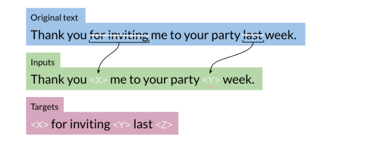
For example, you represent the “for inviting” with <X> and last with <Y> then the model predicts what the X should be and what the Y should be. This is exactly what we saw in the BERT loss. You can also mask out a few positions, not just one. The loss is only on the mask for BERT, for T5 it is on the target.

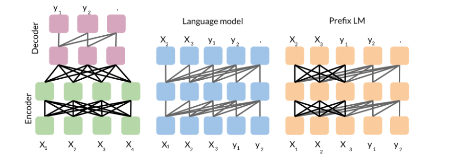
So we start with the basic encoder-decoder representation. There you have a fully visible attention in the encoder and then causal attention in the decoder. So light gray lines correspond to causal masking. And dark gray lines correspond to the fully visible masking.

In the middle we have the language model which consists of a single transformer layer stack. And it’s being fed the concatenation of the inputs and the target. So it uses causal masking throughout as you can see because they’re all gray lines. And you have X1 going inside, you get X2, X2 goes into the model and you get X3 and so forth.

To the right, we have prefix language model which corresponds to allowing fully visible masking over the inputs as you can see with the dark arrows. And then causal masking in the rest.

Multi-Task Training Strategy

Welcome. You will now see how you can train one
model to get you very good results on several NLP tasks. When training such a model, we usually
append a tag to notify whether we’re training on either machine translation,
question answering, summarization, sentiment,
or some other type of task. Let’s see how you can use this
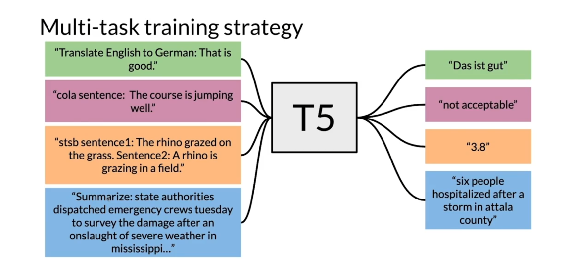
in your own applications. >> Speaker 2: So the multitask
training strategy works as follow. So if you want to translate from English
to German, you append the prefix translate English to German, and it gives
you the corresponding translation. For cola sentence like,
the course is jumping well, and it says it’s not acceptable because
it’s grammatically incorrect. If you have two sentences and
you want to identify their similarity, you put in the stsp sentence 1, and then sentence 2 inside over here,
sentence 1, sentence 2. And then you get the corresponding score. If you want to summarize, you add
the summarize prefix to the article or the text you want to summarize and
it gives you the summary.

STSB（Semantic Textual Similarity Benchmark）是一个用于衡量两个文本片段之间语义相似性的基准数据集。在STSB数据集中，每个样本包含两个句子（sentence1和sentence2）以及一个相似性分数（similarity score），表示这两个句子之间的语义相似程度。

因此，当提到STSB数据集中的sentence1时，指的是数据集中的第一个句子，用于与sentence2进行比较以计算语义相似性分数。 STSB数据集通常用于训练和评估文本相似度模型，以便这些模型能够根据两个文本片段之间的语义相似程度对它们进行比较。

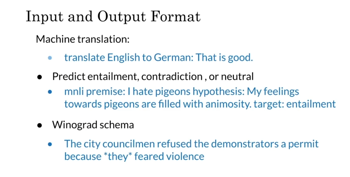
So this is how it works. Inputs and outputs format, so
for machine translation you just do translate blank to blank and
you add the sentence. To predict entailments, contradiction,
or whether it’s neutral, you would feed in something as follows,
so nnli premise, I hate pigeons, then the hypothesis, my feelings towards
pigeons are filled with animosity, and the target is entailment. So basically over here, this is going to
try to learn the overall structure of entailment, and
by feeding in the entire thing, the model would have full visibility
over the entire input, and then it would be tasked with marking a classification
by outputting the word entailment. So it is easy for the model to learn
to predict one of the correct class labels given the task prefix mnli,
in this case. If you know the main difference
between prefix LM and the BERT architecture is that
the classifier is integrated to the output layer of the transformer
decoder in the prefix LM. And over here you have
the Winograd schema, which is another way to predict whether a
pronoun, for example, over here, the city councilmen refused the demonstrators
a permit because they feared violence.

Winograd schema是一种用于测试自然语言处理系统理解普遍知识和推理能力的句子。这些句子由一个关键词和一个代词组成，根据关键词的不同，代词的指代也会不同，需要系统根据句子的上下文和常识进行正确的指代。

Winograd schema最早由计算机科学家Terry Winograd提出，被认为是对自然语言理解的一种较为困难的测试。这种测试通过评估系统是否能够正确理解和推理句子中的逻辑关系和语义含义来评估其智能程度。Winograd schema在评估人工智能系统的语言理解能力和推理能力方面具有重要意义，被广泛应用于自然语言处理和人工智能领域。

So you’re going to feed
this into your model, and then it will be tasked to predict
they as the city councilmen.

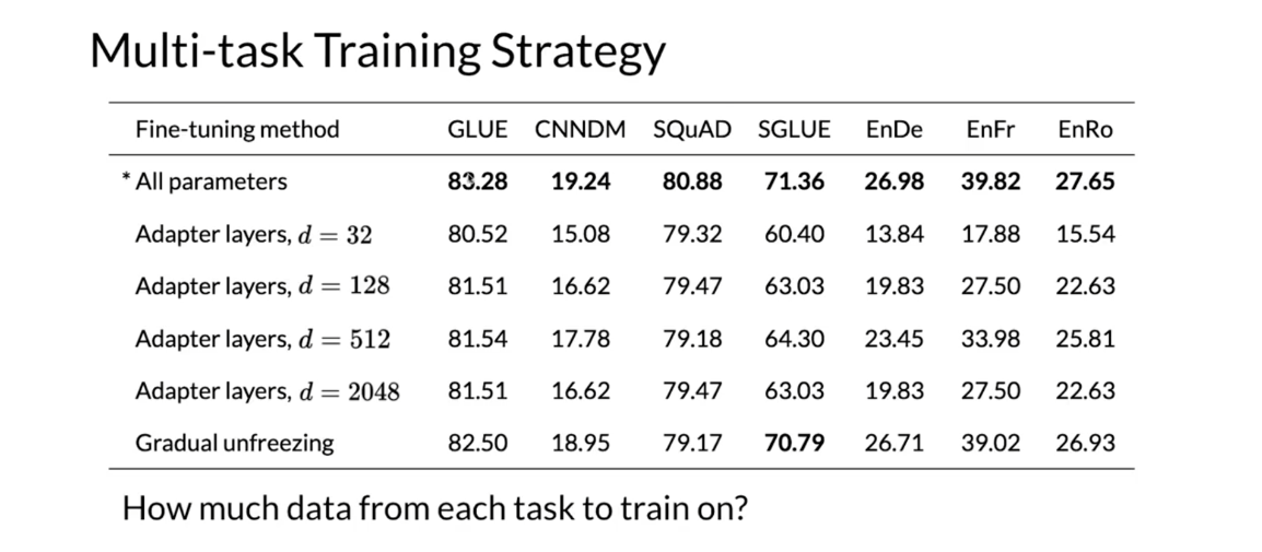
So for multi-task training strategy, this
is a table found in the original paper, and we’ll talk about what
the GLUE benchmark is, and these other benchmarks,
you can check them out. But for the purpose of this week,
we’ll be focusing on the GLUE benchmark, which would be the next video. And we’ll talk about adapter layers and
gradual unfreezing. But these are the scores reported,
and you can see that the T5 paper actually reaches states
of the art in many tasks. So how much data from
each task you train on?

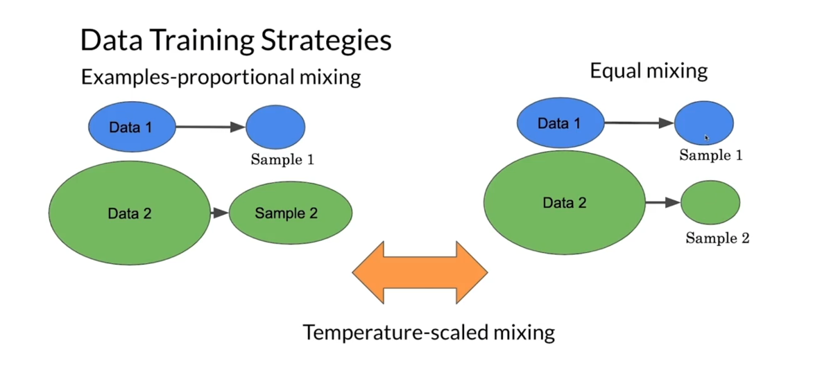
So for the data training strategies,
there is examples proportional mixing, and in this case, what you end up doing,
you take an equal proportion, say, like 10% from each
data that you have. And if the first data sets, for
example, blue, you take 10% of this, then you’ll get 10% over here,
10% of this is larger, and 10% is just a random number I picked,
but you get the point. For the other type of data
training strategy is equal mixing, so regardless of the size of each data,
you take an equal sample. And then there is something in the middle
called temperature-scaled mixing, where you try to play with the parameters
to get something in between.

Now, we’ll talk about gradual
unfreezing versus adapter layers. So in gradual unfreezing,
what ends up happening, you unfreeze one layer at a time. So you say this is your neural network,
unfreezing the last one, you fine-tune using that, you keep the
others fixed, then unfreezing this one, and then you unfreeze this one, so
you keep unfreezing each layer. And for the adapter layers, you basically, add a neural network to each feed-forward
in each block of the transformer. And then, these new feed-forward networks, they’re designed so that the output
dimension matches the input. And this allows them to be inserted
without having any structural change. When fine-tuning only these
new adapter layers and the layer normalization
parameters are being updated.

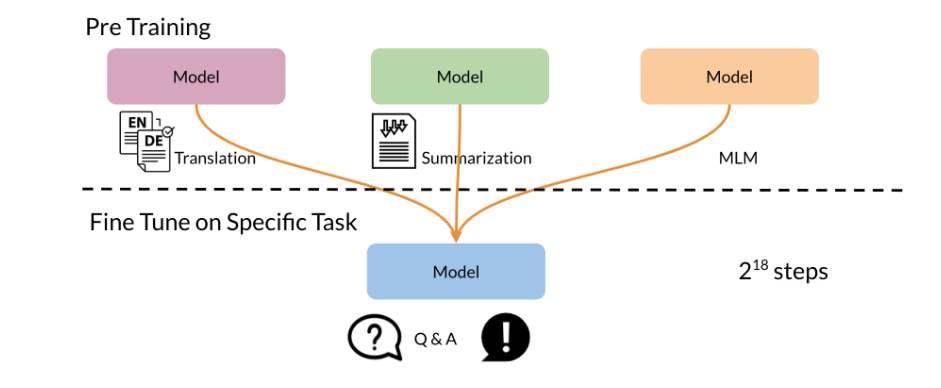
So we’ll talk now a bit
more about fine-tuning. The approach that’s usually being used
here has the goal of training a single model that can simultaneously perform
many tasks at once, for example, the model, most of its parameters
are shared across all of the tasks. And we might train a single model on many
tasks, but when reporting performance, we can select a different checkpoint for
each task. So over here, the task could be
like translation, summarization, or masked language modeling. And they do the train in 2
to the power of 18 steps. >> Speaker 1: You learned about
multiple training strategies used for your transformer model. Now, that you know how to train this
model, you need the way to evaluate it. Concretely, you’ll be evaluating it using
the GLUE benchmark, which stands for General Language Understanding Evaluation
benchmark. See you there.

Gradual unfreezing是一种用于微调预训练语言模型的技术，特别是在处理少量标记数据时非常有效。在这种技术中，模型的不同层在微调过程中逐渐解冻（unfreeze），允许这些层的权重进行调整，以便适应特定任务的数据。

具体来说，gradual unfreezing通常遵循以下步骤：

1. 冻结所有层：首先，将预训练模型中的所有层都冻结，使其权重在微调过程中不会更新。

2. 解冻顶层：然后，只解冻模型的顶层（通常是最后几个层），允许这些层的权重在微调过程中进行调整，而其他层仍保持冻结状态。

3. 微调顶层：使用少量的标记数据对解冻的顶层进行微调，以适应特定的任务。

4. 逐层解冻：接下来，逐渐解冻模型的更多层，每次解冻一层或一组层，并使用更多的标记数据对解冻的层进行微调。

5. 完全微调：最后，将所有层都解冻，并使用全部的标记数据对整个模型进行微调。

gradual unfreezing的优点在于，它可以有效地利用有限的标记数据来微调语言模型，避免在微调过程中过度调整预训练模型的权重，从而提高了微调的效果和泛化能力。

Adapter layers是一种用于在预训练语言模型中进行参数微调的轻量级结构。它们被设计用于在不修改整个模型架构的情况下向模型添加新任务。Adapter layers通常位于预训练模型的每个层之后，用于在特定任务上微调模型。

Adapter layers的主要特点包括：

1. 轻量级：Adapter layers通常包含一个小的全连接层和一个非线性激活函数，参数数量相对较少，使得在添加新任务时不会显著增加模型的复杂度和计算成本。

2. 复用预训练模型：通过使用Adapter layers，可以保持预训练模型的大部分参数不变，只微调添加的Adapter参数，从而可以更好地利用预训练模型学到的知识。

3. 任务特定性：每个Adapter layer可以学习适应特定任务的表示，从而使得模型可以在不同的任务上共享预训练的表示，同时在各个任务上保持较好的性能。

4. 可插拔性：由于Adapter layers的结构轻量级且模块化，可以方便地添加或删除Adapter layers来适应不同的任务需求，而无需重新训练整个模型。

总的来说，Adapter layers为在预训练语言模型上进行参数微调提供了一种灵活且高效的方法，可以有效地在各种自然语言处理任务上提高模型的性能。

GLUE Benchmark

I will show you one of the most commonly
used Benchmarks in natural language processing. Specifically, you’ll learn
about the GLUE Benchmark. This is used to train, evaluate, analyze NLP tasks. Let’s take a look at this
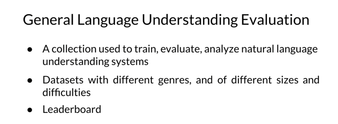
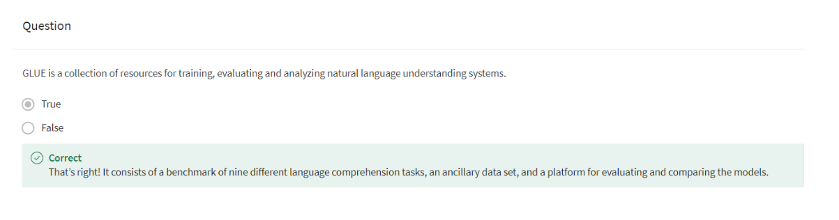
in some more detail. The glue benchmark stands for General Language
Understanding Evaluation. It is basically a collection
that is used to train, evaluate, analyze natural
language understanding systems. It has a lot of datasets
and each dataset has several genres and there are different sizes and
different difficulties. Some of them are, for example, used for co-reference
resolution. Others are just used for
simple sentiment analysis, others are used for question
answering, and so forth. It is used with a leaderboard, so people can use
the datasets and see how well their models
perform compared to others.

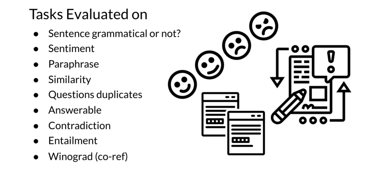
Tasks evaluated on could be, for example, sentence
grammatical or not. For example, if a sentence
makes sense or it does not, is going to be
used on sentiment, it could be used to
paraphrase some texts, it could be used on similarity,
on question duplicates. Whether a question is
answerable or not, whether it’s a contradiction,
whether it’s entailment. Also, for the Winograd schema, which is basically
trying to identify whether a pronoun refers to a certain noun
or to another noun.

It’s used to drive research. As I said, that
researchers usually use the GLUE as a benchmark. It is also a model agnostic, so it doesn’t matter
which model you use. Just evaluate on GLUE and see how well your
model performs. Finally, it allows you to make use of transfer learning
because you have access to several datasets and you can learn
certain things from different datasets
that will help you evaluate on a completely
new datasets within GLUE. You now know not only how to implement states
of the art models, but you also know how
to evaluate them. In the next video, I’ll be talking about
question answering and I’ll show you
how you can use these models to build a sophisticated QA system.
I’ll see you there.

Lab: SentencePiece and BPE

In order to process text in neural network models it is first required to encode text as numbers with ids, since the tensor operations act on numbers. Finally, if the output of the network is to be words, it is required to decode the predicted tokens ids back to text.

SentencePiece and BPE

Introduction to Tokenization

In order to process text in neural network models it is first required to encode text as numbers with ids, since the tensor operations act on numbers. Finally, if the output of the network is to be words, it is required to decode the predicted tokens ids back to text.

To encode text, the first decision that has to be made is to what level of granularity are we going to consider the text? Because ultimately, from these tokens, features are going to be created about them. Many different experiments have been carried out using words, morphological units, phonemic units or characters as tokens. For example,

• Tokens are tricky. (raw text)
• Tokens are tricky . (words)
• Token s _ are _ trick _ y . (morphemes)
• t oʊ k ə n z _ ɑː _ ˈt r ɪ k i. (phonemes, for STT)
• T o k e n s _ a r e _ t r i c k y . (character)

But how to identify these units, such as words, is largely determined by the language they come from. For example, in many European languages a space is used to separate words, while in some Asian languages there are no spaces between words. Compare English and Mandarin.

• Tokens are tricky. (original sentence)
• 标记很棘手 (Mandarin)
• Biāojì hěn jíshǒu (pinyin)
• 标记 很 棘手 (Mandarin with spaces)

So, the ability to tokenize, i.e. split text into meaningful fundamental units, is not always straight-forward.

Also, there are practical issues of how large our vocabulary of words, vocab_size, should be, considering memory limitations vs. coverage. A compromise may be need to be made between:

• the finest-grained models employing characters which can be memory intensive and
• more computationally efficient subword units such as n-grams or larger units.

In SentencePiece unicode characters are grouped together using either a unigram language model (used in this week’s assignment) or BPE, byte-pair encoding. We will discuss BPE, since BERT and many of its variants use a modified version of BPE and its pseudocode is easy to implement and understand… hopefully!

SentencePiece Preprocessing

NFKC Normalization

Unsurprisingly, even using unicode to initially tokenize text can be ambiguous, e.g.,

eaccent = '\u00E9'
e_accent = '\u0065\u0301'
print(f'{eaccent} = {e_accent} : {eaccent == e_accent}')

Output

é = é : False

SentencePiece uses the Unicode standard normalization form, NFKC, so this isn’t an issue. Looking at the example from above but with normalization:

from unicodedata import normalize

norm_eaccent = normalize('NFKC', '\u00E9')
norm_e_accent = normalize('NFKC', '\u0065\u0301')
print(f'{norm_eaccent} = {norm_e_accent} : {norm_eaccent == norm_e_accent}')

Output

é = é : True

Normalization has actually changed the unicode code point (unicode unique id) for one of these two characters.

def get_hex_encoding(s):
    return ' '.join(hex(ord(c)) for c in s)

def print_string_and_encoding(s):
    print(f'{s} : {get_hex_encoding(s)}') 

for s in [eaccent, e_accent, norm_eaccent, norm_e_accent]:
    print_string_and_encoding(s)

Output

é : 0xe9
é : 0x65 0x301
é : 0xe9
é : 0xe9

This normalization has other side effects which may be considered useful such as converting curly quotes “ to " their ASCII equivalent. (^*Although we now lose directionality of the quote…)

Lossless Tokenization

SentencePiece also ensures that when you tokenize your data and detokenize your data the original position of white space is preserved. However, tabs and newlines are converted to spaces.

To ensure this lossless tokenization, SentencePiece replaces white space with _ (U+2581). So that a simple join of the tokens by replacing underscores with spaces can restore the white space, even if there are consecutive symbols. But remember first to normalize and then replace spaces with _ (U+2581).

​

s = 'Tokenization is hard.'
sn = normalize('NFKC', s)
sn_ = sn.replace(' ', '\u2581')

print(get_hex_encoding(s))
print(get_hex_encoding(sn))
print(get_hex_encoding(sn_))

Output

0x54 0x6f 0x6b 0x65 0x6e 0x69 0x7a 0x61 0x74 0x69 0x6f 0x6e 0x20 0x69 0x73 0x20 0x68 0x61 0x72 0x64 0x2e
0x54 0x6f 0x6b 0x65 0x6e 0x69 0x7a 0x61 0x74 0x69 0x6f 0x6e 0x20 0x69 0x73 0x20 0x68 0x61 0x72 0x64 0x2e
0x54 0x6f 0x6b 0x65 0x6e 0x69 0x7a 0x61 0x74 0x69 0x6f 0x6e 0x2581 0x69 0x73 0x2581 0x68 0x61 0x72 0x64 0x2e

BPE Algorithm

After discussing the preprocessing that SentencePiece performs, you will get the data, preprocess it, and apply the BPE algorithm. You will see how this reproduces the tokenization produced by training SentencePiece on the example dataset (from this week’s assignment).

Preparing our Data

First, you get the Squad data and process it as above.

import ast

def convert_json_examples_to_text(filepath):
    example_jsons = list(map(ast.literal_eval, open(filepath))) # Read in the json from the example file
    texts = [example_json['text'].decode('utf-8') for example_json in example_jsons] # Decode the byte sequences
    text = '\n\n'.join(texts)       # Separate different articles by two newlines
    text = normalize('NFKC', text)  # Normalize the text

    with open('example.txt', 'w') as fw:
        fw.write(text)
    
    return text

text = convert_json_examples_to_text('./data/data.txt')
print(text[:900])

Output

Beginners BBQ Class Taking Place in Missoula!
Do you want to get better at making delicious BBQ? You will have the opportunity, put this on your calendar now. Thursday, September 22nd join World Class BBQ Champion, Tony Balay from Lonestar Smoke Rangers. He will be teaching a beginner level class for everyone who wants to get better with their culinary skills.
He will teach you everything you need to know to compete in a KCBS BBQ competition, including techniques, recipes, timelines, meat selection and trimming, plus smoker and fire information.
The cost to be in the class is $35 per person, and for spectators it is free. Included in the cost will be either a t-shirt or apron and you will be tasting samples of each meat that is prepared.

Discussion in 'Mac OS X Lion (10.7)' started by axboi87, Jan 20, 2012.
I've got a 500gb internal drive and a 240gb SSD.
When trying to restore using di

In the algorithm the vocab variable is actually a frequency dictionary of the words. Those words have been prepended with an underscore to indicate that they are the beginning of a word. Finally, the characters have been delimited by spaces so that the BPE algorithm can group the most common characters together in the dictionary in a greedy fashion. You will see how that is done shortly.

from collections import Counter

vocab = Counter(['\u2581' + word for word in text.split()])
vocab = {' '.join([l for l in word]): freq for word, freq in vocab.items()}

解释：vocab = {' '.join([l for l in word]): freq for word, freq in vocab.items()}

这段代码是将一个词典（vocab）中的每个单词按照字母拆分成一个字母的序列，并将序列中的字母用空格分隔开，然后将拆分后的序列作为键，原来单词对应的频率作为值重新构建成一个新的词典。

具体来说，假设原始的词典（vocab）如下所示：

{
  'low': 5,
  'lower': 3,
  'newest': 2,
  'widest': 4
}

经过这段代码处理后，生成的新词典如下所示：

{
  'l o w': 5,
  'l o w e r': 3,
  'n e w e s t': 2,
  'w i d e s t': 4
}

这种处理方式通常用于将单词拆分成子词（例如，按照字母级别拆分），以便后续进行一些文本处理或者特征提取操作。

def show_vocab(vocab, end='\n', limit=20):
    """Show word frequencys in vocab up to the limit number of words"""
    shown = 0
    for word, freq in vocab.items():
        print(f'{word}: {freq}', end=end)
        shown +=1
        if shown > limit:
            break

show_vocab(vocab)

Output

▁ B e g i n n e r s: 1
▁ B B Q: 3
▁ C l a s s: 2
▁ T a k i n g: 1
▁ P l a c e: 1
▁ i n: 15
▁ M i s s o u l a !: 1
▁ D o: 1
▁ y o u: 13
▁ w a n t: 1
▁ t o: 33
▁ g e t: 2
▁ b e t t e r: 2
▁ a t: 1
▁ m a k i n g: 2
▁ d e l i c i o u s: 1
▁ B B Q ?: 1
▁ Y o u: 1
▁ w i l l: 6
▁ h a v e: 4
▁ t h e: 31

You check the size of the vocabulary (frequency dictionary) because this is the one hyperparameter that BPE depends on crucially on how far it breaks up a word into SentencePieces. It turns out that for your trained model on the small dataset that 60% of 455 merges of the most frequent characters need to be done to reproduce the upperlimit of a 32K vocab_size over the entire corpus of examples.

print(f'Total number of unique words: {len(vocab)}')
print(f'Number of merges required to reproduce SentencePiece training on the whole corpus: {int(0.60*len(vocab))}')

Output

Total number of unique words: 455
Number of merges required to reproduce SentencePiece training on the whole corpus: 273

BPE Algorithm

Directly from the BPE paper you have the following algorithm.

import re, collections

def get_stats(vocab):
    pairs = collections.defaultdict(int)
    for word, freq in vocab.items():
        symbols = word.split()
        for i in range(len(symbols) - 1):
            pairs[symbols[i], symbols[i+1]] += freq
    return pairs

def merge_vocab(pair, v_in):
    v_out = {}
    bigram = re.escape(' '.join(pair))
    p = re.compile(r'(?<!\S)' + bigram + r'(?!\S)')
    for word in v_in:
        w_out = p.sub(''.join(pair), word)
        v_out[w_out] = v_in[word]
    return v_out

def get_sentence_piece_vocab(vocab, frac_merges=0.60):
    sp_vocab = vocab.copy()
    num_merges = int(len(sp_vocab)*frac_merges)
    
    for i in range(num_merges):
        pairs = get_stats(sp_vocab)
        best = max(pairs, key=pairs.get)
        sp_vocab = merge_vocab(best, sp_vocab)

    return sp_vocab

BPE（Byte Pair Encoding）算法是一种数据压缩算法，也被广泛应用于自然语言处理中的子词分割和词形还原等任务中。BPE算法由Philip Gage于1994年提出，后来被Sennrich等人在2016年应用于神经机器翻译中。

BPE算法的基本思想是通过迭代地合并数据中最频繁出现的一对连续字节对（byte pair）来构建一个字节对词典，从而实现数据的压缩。在自然语言处理中，字节对通常被视为字符对，因此BPE算法实际上是一种基于字符的合并算法。

BPE算法的步骤如下：

1. 初始化：将每个字符视为一个单独的子词。

2. 统计频率：统计数据中所有连续字符对（或字节对）的频率。

3. 合并频率最高的字符对：将频率最高的字符对合并为一个新的字符，并将这个新字符加入到词典中。

4. 更新词典：更新词典中的所有子词，将其中包含被合并的字符对的子词替换为新的字符。

5. 重复步骤3和步骤4，直到达到预设的合并次数或者词典大小。

在自然语言处理中，BPE算法通常用于学习一种能够表示单词和子词的词典，从而在词典中生成更少、更具有信息量的单词和子词，以便于模型处理。例如，在神经机器翻译中，BPE算法可以用来构建源语言和目标语言的子词词典，以便于模型处理未登录词和低频词。

To understand what’s going on first take a look at the third function get_sentence_piece_vocab. It takes in the current vocab word-frequency dictionary and the fraction, frac_merges, of the total vocab_size to merge characters in the words of the dictionary, num_merges times. Then for each merge operation it get_stats on how many of each pair of character sequences there are. It gets the most frequent pair of symbols as the best pair. Then it merges that pair of symbols (removes the space between them) in each word in the vocab that contains this best (= pair). Consequently, merge_vocab creates a new vocab, v_out. This process is repeated num_merges times and the result is the set of SentencePieces (keys of the final sp_vocab).

Additional Discussion of BPE Algorithm

Please feel free to skip the below if the above description was enough.

In a little more detail you can see in get_stats you initially create a list of bigram (two character sequence) frequencies from the vocabulary. Later, this may include trigrams, quadgrams, etc. Note that the key of the pairs frequency dictionary is actually a 2-tuple, which is just shorthand notation for a pair.

In merge_vocab you take in an individual pair (of character sequences, note this is the most frequency best pair) and the current vocab as v_in. You create a new vocab, v_out, from the old by joining together the characters in the pair (removing the space), if they are present in a word of the dictionary.

Warning: the expression (?<!\S) means that either a whitespace character follows before the bigram or there is nothing before the bigram (it is the beginning of the word), similarly for (?!\S) for preceding whitespace or the end of the word.

sp_vocab = get_sentence_piece_vocab(vocab)
show_vocab(sp_vocab) 

Output

▁B e g in n ers: 1
▁BBQ: 3
▁Cl ass: 2
▁T ak ing: 1
▁P la ce: 1
▁in: 15
▁M is s ou la !: 1
▁D o: 1
▁you: 13
▁w an t: 1
▁to: 33
▁g et: 2
▁be t ter: 2
▁a t: 1
▁mak ing: 2
▁d e l ic i ou s: 1
▁BBQ ?: 1
▁ Y ou: 1
▁will: 6
▁have: 4
▁the: 31

Train SentencePiece BPE Tokenizer on Example Data

Explore SentencePiece Model

First, explore the SentencePiece model provided with this week’s assignment. Remember you can always use Python’s built in help command to see the documentation for any object or method.

import sentencepiece as spm
sp = spm.SentencePieceProcessor(model_file='./data/sentencepiece.model')

Try it out on the first sentence of the example text.

s0 = 'Beginners BBQ Class Taking Place in Missoula!'

# encode: text => id
print(sp.encode_as_pieces(s0))
print(sp.encode_as_ids(s0))

# decode: id => text
print(sp.decode_pieces(sp.encode_as_pieces(s0)))
print(sp.decode_ids([12847, 277]))

Output

['▁Beginn', 'ers', '▁BBQ', '▁Class', '▁', 'Taking', '▁Place', '▁in', '▁Miss', 'oul', 'a', '!']
[12847, 277, 15068, 4501, 3, 12297, 3399, 16, 5964, 7115, 9, 55]
Beginners BBQ Class Taking Place in Missoula!
Beginners

Notice how SentencePiece breaks the words into seemingly odd parts, but you have seen something similar with BPE. But how close was the model trained on the whole corpus of examples with a vocab_size of 32,000 instead of 455? Here you can also test what happens to white space, like ‘\n’.

But first note that SentencePiece encodes the SentencePieces, the tokens, and has reserved some of the ids as can be seen in this week’s assignment.

uid = 15068
spiece = "\u2581BBQ"
unknown = "__MUST_BE_UNKNOWN__"

# id <=> piece conversion
print(f'SentencePiece for ID {uid}: {sp.id_to_piece(uid)}')
print(f'ID for Sentence Piece {spiece}: {sp.piece_to_id(spiece)}')

# returns 0 for unknown tokens (we can change the id for UNK)
print(f'ID for unknown text {unknown}: {sp.piece_to_id(unknown)}')

Output

SentencePiece for ID 15068: ▁BBQ
ID for Sentence Piece ▁BBQ: 15068
ID for unknown text __MUST_BE_UNKNOWN__: 2

print(f'Beginning of sentence id: {sp.bos_id()}')
print(f'Pad id: {sp.pad_id()}')
print(f'End of sentence id: {sp.eos_id()}')
print(f'Unknown id: {sp.unk_id()}')
print(f'Vocab size: {sp.vocab_size()}')

Output

Beginning of sentence id: -1
Pad id: 0
End of sentence id: 1
Unknown id: 2
Vocab size: 32000

You can also check what are the ids for the first part and last part of the vocabulary.

print('\nId\tSentP\tControl?')
print('------------------------')
# <unk>, <s>, </s> are defined by default. Their ids are (0, 1, 2)
# <s> and </s> are defined as 'control' symbol.
for uid in range(10):
    print(uid, sp.id_to_piece(uid), sp.is_control(uid), sep='\t')
    
# for uid in range(sp.vocab_size()-10,sp.vocab_size()):
#     print(uid, sp.id_to_piece(uid), sp.is_control(uid), sep='\t')

Output

Id	SentP	Control?
------------------------
0	<pad>	True
1	</s>	True
2	<unk>	False
3	▁	False
4	X	False
5	.	False
6	,	False
7	s	False
8	▁the	False
9	a	False

Train SentencePiece BPE model with our example.txt

Finally, train your own BPE model directly from the SentencePiece library and compare it to the results of the implemention of the algorithm from the BPE paper itself.

spm.SentencePieceTrainer.train('--input=example.txt --model_prefix=example_bpe --vocab_size=450 --model_type=bpe')
sp_bpe = spm.SentencePieceProcessor()
sp_bpe.load('example_bpe.model')

print('*** BPE ***')
print(sp_bpe.encode_as_pieces(s0))

Output

*** BPE ***
['▁B', 'e', 'ginn', 'ers', '▁BBQ', '▁Cl', 'ass', '▁T', 'ak', 'ing', '▁P', 'la', 'ce', '▁in', '▁M', 'is', 's', 'ou', 'la', '!']

show_vocab(sp_vocab, end = ', ')

Output

▁B e g in n ers: 1, ▁BBQ: 3, ▁Cl ass: 2, ▁T ak ing: 1, ▁P la ce: 1, ▁in: 15, ▁M is s ou la !: 1, ▁D o: 1, ▁you: 13, ▁w an t: 1, ▁to: 33, ▁g et: 2, ▁be t ter: 2, ▁a t: 1, ▁mak ing: 2, ▁d e l ic i ou s: 1, ▁BBQ ?: 1, ▁ Y ou: 1, ▁will: 6, ▁have: 4, ▁the: 31, 

The implementation of BPE’s code from the paper matches up pretty well with the library itself! The differences are probably accounted for by the vocab_size. There is also another technical difference in that in the SentencePiece implementation of BPE a priority queue is used to more efficiently keep track of the best pairs. Actually, there is a priority queue in the Python standard library called heapq if you would like to give that a try below!

Optionally try to implement BPE using a priority queue below

from heapq import heappush, heappop

def heapsort(iterable):
    h = []
    for value in iterable:
        heappush(h, value)
    return [heappop(h) for i in range(len(h))]

a = [1,4,3,1,3,2,1,4,2]
heapsort(a)

Output

[1, 1, 1, 2, 2, 3, 3, 4, 4]

For a more extensive example consider looking at the SentencePiece repo. The last few sections of this code were repurposed from that tutorial. Thanks for your participation! Next stop BERT and T5!

Welcome to Hugging Face 🤗

When it comes to building real-world applications with Transformer models, the vast majority of industry practitioners are working with pre-trained models, rather than building and training them from scratch.

In order to provide you with an opportunity to work with some pre-trained Transformer models, we at DeepLearning.AI have partnered with Hugging Face to create the upcoming videos and labs, where you can get some hands-on practice doing things just like people are doing in industry every day.

Move on to the next video to learn more about all the amazing open-source tools and resources that Hugging Face provides and after that, we’ll get into the labs.

Hugging Face Introduction

Hugging Face I

Hugging Face II

Hugging Face III

Lab: Question Answering with HuggingFace - Using a base model

Question Answering with BERT and HuggingFace

You’ve seen how to use BERT and other transformer models for a wide range of natural language tasks, including machine translation, summarization, and question answering. Transformers have become the standard model for NLP, similar to convolutional models in computer vision. And all started with Attention!

In practice, you’ll rarely train a transformer model from scratch. Transformers tend to be very large, so they take time, money, and lots of data to train fully. Instead, you’ll want to start with a pre-trained model and fine-tune it with your dataset if you need to.

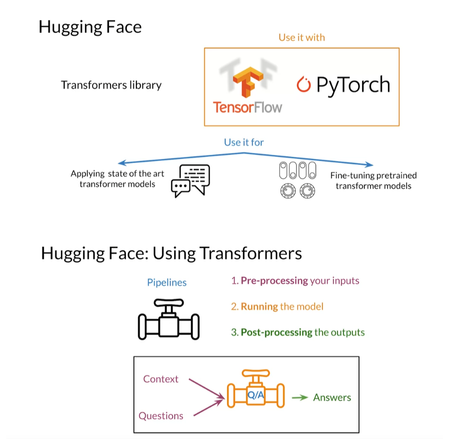
Hugging Face (🤗) is the best resource for pre-trained transformers. Their open-source libraries simplify downloading and using transformer models like BERT, T5, and GPT-2. And the best part, you can use them alongside either TensorFlow, PyTorch or Flax.

In this notebook, you’ll use 🤗 transformers to use the DistilBERT model for question answering.

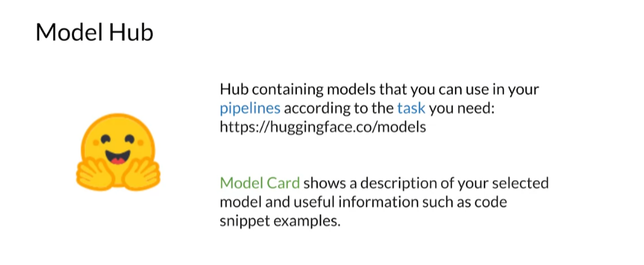
Pipelines

Before fine-tuning a model, you will look at the pipelines from Hugging Face to use pre-trained transformer models for specific tasks. The transformers library provides pipelines for popular tasks like sentiment analysis, summarization, and text generation. A pipeline consists of a tokenizer, a model, and the model configuration. All these are packaged together into an easy-to-use object. Hugging Face makes life easier.

Pipelines are intended to be used without fine-tuning and will often be immediately helpful in your projects. For example, transformers provides a pipeline for question answering that you can directly use to answer your questions if you give some context. Let’s see how to do just that.

You will import pipeline from transformers for creating pipelines.

import os
os.environ['TF_CPP_MIN_LOG_LEVEL'] = '3'

from transformers import pipeline

Now, you will create the pipeline for question-answering, which uses the DistilBert model for extractive question answering (i.e., answering questions with the exact wording provided in the context).

# The task "question-answering" will return a QuestionAnsweringPipeline object
question_answerer = pipeline(task="question-answering", model="distilbert-base-cased-distilled-squad")

Notice that this environment already has the model stored in the directory distilbert-base-cased-distilled-squad. However if you were to run that exact code on your local computer, Huggingface will download the model for you, which is a great feature!

After running the last cell, you have a pipeline for performing question answering given a context string. The pipeline question_answerer you just created needs you to pass the question and context as strings. It returns an answer to the question from the context you provided. For example, here are the first few paragraphs from the Wikipedia entry for tea that you will use as the context.

context = """
Tea is an aromatic beverage prepared by pouring hot or boiling water over cured or fresh leaves of Camellia sinensis,
an evergreen shrub native to China and East Asia. After water, it is the most widely consumed drink in the world.
There are many different types of tea; some, like Chinese greens and Darjeeling, have a cooling, slightly bitter,
and astringent flavour, while others have vastly different profiles that include sweet, nutty, floral, or grassy
notes. Tea has a stimulating effect in humans primarily due to its caffeine content.

The tea plant originated in the region encompassing today's Southwest China, Tibet, north Myanmar and Northeast India,
where it was used as a medicinal drink by various ethnic groups. An early credible record of tea drinking dates to
the 3rd century AD, in a medical text written by Hua Tuo. It was popularised as a recreational drink during the
Chinese Tang dynasty, and tea drinking spread to other East Asian countries. Portuguese priests and merchants
introduced it to Europe during the 16th century. During the 17th century, drinking tea became fashionable among the
English, who started to plant tea on a large scale in India.

The term herbal tea refers to drinks not made from Camellia sinensis: infusions of fruit, leaves, or other plant
parts, such as steeps of rosehip, chamomile, or rooibos. These may be called tisanes or herbal infusions to prevent
confusion with 'tea' made from the tea plant.
"""

Now, you can ask your model anything related to that passage. For instance, “Where is tea native to?”.

result = question_answerer(question="Where is tea native to?", context=context)

print(result['answer'])

Output

China and East Asia

You can also pass multiple questions to your pipeline within a list so that you can ask:

• “Where is tea native to?”
• “When was tea discovered?”
• “What is the species name for tea?”

at the same time, and your question-answerer will return all the answers.

questions = ["Where is tea native to?",
             "When was tea discovered?",
             "What is the species name for tea?"]

results = question_answerer(question=questions, context=context)

for q, r in zip(questions, results):
    print(f"{q} \n>> {r['answer']}")

Output

Where is tea native to? 
>> China and East Asia
When was tea discovered? 
>> 3rd century AD
What is the species name for tea? 
>> Camellia sinensis

Although the models used in the Hugging Face pipelines generally give outstanding results, sometimes you will have particular examples where they don’t perform so well. Let’s use the following example with a context string about the Golden Age of Comic Books:

context = """
The Golden Age of Comic Books describes an era of American comic books from the
late 1930s to circa 1950. During this time, modern comic books were first published
and rapidly increased in popularity. The superhero archetype was created and many
well-known characters were introduced, including Superman, Batman, Captain Marvel
(later known as SHAZAM!), Captain America, and Wonder Woman.
Between 1939 and 1941 Detective Comics and its sister company, All-American Publications,
introduced popular superheroes such as Batman and Robin, Wonder Woman, the Flash,
Green Lantern, Doctor Fate, the Atom, Hawkman, Green Arrow and Aquaman.[7] Timely Comics,
the 1940s predecessor of Marvel Comics, had million-selling titles featuring the Human Torch,
the Sub-Mariner, and Captain America.[8]
As comic books grew in popularity, publishers began launching titles that expanded
into a variety of genres. Dell Comics' non-superhero characters (particularly the
licensed Walt Disney animated-character comics) outsold the superhero comics of the day.[12]
The publisher featured licensed movie and literary characters such as Mickey Mouse, Donald Duck,
Roy Rogers and Tarzan.[13] It was during this era that noted Donald Duck writer-artist
Carl Barks rose to prominence.[14] Additionally, MLJ's introduction of Archie Andrews
in Pep Comics #22 (December 1941) gave rise to teen humor comics,[15] with the Archie
Andrews character remaining in print well into the 21st century.[16]
At the same time in Canada, American comic books were prohibited importation under
the War Exchange Conservation Act[17] which restricted the importation of non-essential
goods. As a result, a domestic publishing industry flourished during the duration
of the war which were collectively informally called the Canadian Whites.
The educational comic book Dagwood Splits the Atom used characters from the comic
strip Blondie.[18] According to historian Michael A. Amundson, appealing comic-book
characters helped ease young readers' fear of nuclear war and neutralize anxiety
about the questions posed by atomic power.[19] It was during this period that long-running
humor comics debuted, including EC's Mad and Carl Barks' Uncle Scrooge in Dell's Four
Color Comics (both in 1952).[20][21]
"""

Let’s ask the following question: “What popular superheroes were introduced between 1939 and 1941?” The answer is in the fourth paragraph of the context string.

question = "What popular superheroes were introduced between 1939 and 1941?"

result = question_answerer(question=question, context=context)
print(result['answer'])

Output

teen humor comics

Here, the answer should be:
“Batman and Robin, Wonder Woman, the Flash,
Green Lantern, Doctor Fate, the Atom, Hawkman, Green Arrow, and Aquaman”. Instead, the pipeline returned a different answer. You can even try different question wordings:

• “What superheroes were introduced between 1939 and 1941?”
• “What comic book characters were created between 1939 and 1941?”
• “What well-known characters were created between 1939 and 1941?”
• “What well-known superheroes were introduced between 1939 and 1941 by Detective Comics?”

and you will only get incorrect answers.

questions = ["What popular superheroes were introduced between 1939 and 1941?",
             "What superheroes were introduced between 1939 and 1941 by Detective Comics and its sister company?",
             "What comic book characters were created between 1939 and 1941?",
             "What well-known characters were created between 1939 and 1941?",
             "What well-known superheroes were introduced between 1939 and 1941 by Detective Comics?"]

results = question_answerer(question=questions, context=context)

for q, r in zip(questions, results):
    print(f"{q} \n>> {r['answer']}")

Output

What popular superheroes were introduced between 1939 and 1941? 
>> teen humor comics
What superheroes were introduced between 1939 and 1941 by Detective Comics and its sister company? 
>> Archie Andrews
What comic book characters were created between 1939 and 1941? 
>> Archie
Andrews
What well-known characters were created between 1939 and 1941? 
>> Archie
Andrews
What well-known superheroes were introduced between 1939 and 1941 by Detective Comics? 
>> Archie Andrews

It seems like this model is a huge fan of Archie Andrews. It even considers him a superhero!

The example that fooled your question_answerer belongs to the TyDi QA dataset, a dataset from Google for question/answering in diverse languages. To achieve better results when you know that the pipeline isn’t working as it should, you need to consider fine-tuning your model.

In the next ungraded lab, you will get the chance to fine-tune the DistilBert model using the TyDi QA dataset.

Lab: Question Answering with HuggingFace 2 - Fine-tuning a model

Question Answering with BERT and HuggingFace 🤗 (Fine-tuning)

In the previous Hugging Face ungraded lab, you saw how to use the pipeline objects to use transformer models for NLP tasks. In that lab, the model didn’t output the desired answers to a series of precise questions for a context related to the history of comic books.

In this lab, you will fine-tune the model from that lab to give better answers for that type of context. To do that, you’ll be using the TyDi QA dataset but on a filtered version with only English examples. Additionally, you will use a lot of the tools that Hugging Face has to offer.

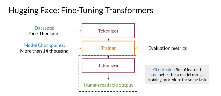
You have to note that, in general, you will fine-tune general-purpose transformer models to work for specific tasks. However, fine-tuning a general-purpose model can take a lot of time. That’s why you will be using the model from the question answering pipeline in this lab.

Begin by importing some libraries and/or objects you will use throughout the lab:

import os
os.environ['TF_CPP_MIN_LOG_LEVEL'] = '3'

import numpy as np

from datasets import load_from_disk
from transformers import AutoTokenizer, AutoModelForQuestionAnswering, Trainer, TrainingArguments

from sklearn.metrics import f1_score

Fine-tuning a BERT model

As you saw in the previous lab, you can use these pipelines as they are. But sometimes, you’ll need something more specific to your problem, or maybe you need it to perform better on your production data. In these cases, you’ll need to fine-tune a model.

Here, you’ll fine-tune a pre-trained DistilBERT model on the TyDi QA dataset.

To fine-tune your model, you will leverage three components provided by Hugging Face:

• Datasets: Library that contains some datasets and different metrics to evaluate the performance of your models.
• Tokenizer: Object in charge of preprocessing your text to be given as input for the transformer models.
• Transformers: Library with the pre-trained model checkpoints and the trainer object.

Datasets

To get the dataset to fine-tune your model, you will use 🤗 Datasets, a lightweight and extensible library to share and access datasets and evaluation metrics for NLP easily. You can download Hugging Face datasets directly using the load_dataset function from the datasets library.

Hugging Face datasets allows to load data in several formats, such as CSV, JSON, text files and even parquet. You can see more about the supported formats in the documentation

A common approach is to use load_dataset and get the full dataset but for this lab you will use a filtered version containing only the English examples, which is already saved in this environment. Since this filtered dataset is saved using the Apache Arrow format, you can read it by using the load_from_disk function.

#The path where the dataset is stored
path = './tydiqa_data/'

#Load Dataset
tydiqa_data = load_from_disk(path)

tydiqa_data

Output

DatasetDict({
    train: Dataset({
        features: ['passage_answer_candidates', 'question_text', 'document_title', 'language', 'annotations', 'document_plaintext', 'document_url'],
        num_rows: 9211
    })
    validation: Dataset({
        features: ['passage_answer_candidates', 'question_text', 'document_title', 'language', 'annotations', 'document_plaintext', 'document_url'],
        num_rows: 1031
    })
})

You can check below that the type of the loaded dataset is a datasets.arrow_dataset.Dataset. This object type corresponds to an Apache Arrow Table that allows creating a hash table that contains the position in memory where data is stored instead of loading the complete dataset into memory. But you don’t have to worry too much about that. It is just an efficient way to work with lots of data.

# Checking the object type for one of the elements in the dataset
type(tydiqa_data['train'])

Output

datasets.arrow_dataset.Dataset

You can also check the structure of the dataset:

tydiqa_data['train']

Output

Dataset({
    features: ['passage_answer_candidates', 'question_text', 'document_title', 'language', 'annotations', 'document_plaintext', 'document_url'],
    num_rows: 9211
})

You can see that each example is like a dictionary object. This dataset consists of questions, contexts, and indices that point to the start and end position of the answer inside the context. You can access the index using the annotations key, which is a kind of dictionary.

idx = 600

# start index
start_index = tydiqa_data['train'][idx]['annotations']['minimal_answers_start_byte'][0]

# end index
end_index = tydiqa_data['train'][idx]['annotations']['minimal_answers_end_byte'][0]

print(f"Question: {tydiqa_data['train'][idx]['question_text']}")
print(f"\nContext (truncated): {tydiqa_data['train'][idx]['document_plaintext'][0:512]} ...")
print(f"\nAnswer: {tydiqa_data['train'][idx]['document_plaintext'][start_index:end_index]}")

Output

Question: What mental effects can a mother experience after childbirth?

Context (truncated): 

Postpartum depression (PPD), also called postnatal depression, is a type of mood disorder associated with childbirth, which can affect both sexes.[1][3] Symptoms may include extreme sadness, low energy, anxiety, crying episodes, irritability, and changes in sleeping or eating patterns.[1] Onset is typically between one week and one month following childbirth.[1] PPD can also negatively affect the newborn child.[2]

While the exact cause of PPD is unclear, the cause is believed to be a combination of physi ...

Answer: Postpartum depression (PPD)

The question answering model predicts a start and endpoint in the context to extract as the answer. That’s why this NLP task is known as extractive question answering.

To train your model, you need to pass start and endpoints as labels. So, you need to implement a function that extracts the start and end positions from the dataset.

The dataset contains unanswerable questions. For these, the start and end indices for the answer are equal to -1.

tydiqa_data['train'][0]['annotations']

Output

{'passage_answer_candidate_index': [-1],
 'minimal_answers_start_byte': [-1],
 'minimal_answers_end_byte': [-1],
 'yes_no_answer': ['NONE']}

Now, you have to flatten the dataset to work with an object with a table structure instead of a dictionary structure. This step facilitates the pre-processing steps.

# Flattening the datasets
flattened_train_data = tydiqa_data['train'].flatten()
flattened_test_data =  tydiqa_data['validation'].flatten()

Also, to make the training more straightforward and faster, we will extract a subset of the train and test datasets. For that purpose, we will use the Hugging Face Dataset object’s method called select(). This method allows you to take some data points by their index. Here, you will select the first 3000 rows but you can play with the number of data points, however, consider that this will increase the training time.

# Selecting a subset of the train dataset
flattened_train_data = flattened_train_data.select(range(3000))

# Selecting a subset of the test dataset
flattened_test_data = flattened_test_data.select(range(1000))

Tokenizers

Now, you will use the tokenizer object from Hugging Face. You can load a tokenizer using different methods. Here, you will retrieve it from the pipeline object you created in the previous Hugging Face lab. With this tokenizer, you can ensure that the tokens you get for the dataset will match the tokens used in the original DistilBERT implementation.

When loading a tokenizer with any method, you must pass the model checkpoint that you want to fine-tune. Here, you are using the'distilbert-base-cased-distilled-squad' checkpoint.

# Import the AutoTokenizer from the transformers library
tokenizer = AutoTokenizer.from_pretrained("distilbert-base-cased-distilled-squad")

# Define max length of sequences in the tokenizer
tokenizer.model_max_length = 512

Given the characteristics of the dataset and the question-answering task, you will need to add some steps to pre-process the data after the tokenization:

1. When there is no answer to a question given a context, you will use the CLS token, a unique token used to represent the start of the sequence.

2. Tokenizers can split a given string into substrings, resulting in a subtoken for each substring, creating misalignment between the list of dataset tags and the labels generated by the tokenizer. Therefore, you will need to align the start and end indices with the tokens associated with the target answer word.

3. Finally, a tokenizer can truncate a very long sequence. So, if the start/end position of an answer is None, you will assume that it was truncated and assign the maximum length of the tokenizer to those positions.

Those three steps are done within the process_samples function defined below.

# Processing samples using the 3 steps described above
def process_samples(sample):
    tokenized_data = tokenizer(sample['document_plaintext'], sample['question_text'], truncation="only_first", padding="max_length")

    input_ids = tokenized_data["input_ids"]

    # We will label impossible answers with the index of the CLS token.
    cls_index = input_ids.index(tokenizer.cls_token_id)

    # If no answers are given, set the cls_index as answer.
    if sample["annotations.minimal_answers_start_byte"][0] == -1:
        start_position = cls_index
        end_position = cls_index
    else:
        # Start/end character index of the answer in the text.
        gold_text = sample["document_plaintext"][sample['annotations.minimal_answers_start_byte'][0]:sample['annotations.minimal_answers_end_byte'][0]]
        start_char = sample["annotations.minimal_answers_start_byte"][0]
        end_char = sample['annotations.minimal_answers_end_byte'][0] #start_char + len(gold_text)

        # sometimes answers are off by a character or two – fix this
        if sample['document_plaintext'][start_char-1:end_char-1] == gold_text:
            start_char = start_char - 1
            end_char = end_char - 1     # When the gold label is off by one character
        elif sample['document_plaintext'][start_char-2:end_char-2] == gold_text:
            start_char = start_char - 2
            end_char = end_char - 2     # When the gold label is off by two characters

        start_token = tokenized_data.char_to_token(start_char)
        end_token = tokenized_data.char_to_token(end_char - 1)

        # if start position is None, the answer passage has been truncated
        if start_token is None:
            start_token = tokenizer.model_max_length
        if end_token is None:
            end_token = tokenizer.model_max_length

        start_position = start_token
        end_position = end_token

    return {'input_ids': tokenized_data['input_ids'],
          'attention_mask': tokenized_data['attention_mask'],
          'start_positions': start_position,
          'end_positions': end_position}

To apply the process_samples function defined above to the whole dataset, you can use the map method as follows:

# Tokenizing and processing the flattened dataset
processed_train_data = flattened_train_data.map(process_samples)
processed_test_data = flattened_test_data.map(process_samples)

Transformers

The last component of Hugging Face that is useful for fine-tuning a transformer corresponds to the pre-trained models you can access in multiple ways.

For this lab, you will use the same model from the question-answering pipeline that you loaded in the previous lab.

# Import the AutoModelForQuestionAnswering for the pre-trained model. You will only fine tune the head of the model
model = AutoModelForQuestionAnswering.from_pretrained("distilbert-base-cased-distilled-squad")

Now, you can take the necessary columns from the datasets to train/test and return them as Pytorch Tensors.

columns_to_return = ['input_ids','attention_mask', 'start_positions', 'end_positions']

processed_train_data.set_format(type='pt', columns=columns_to_return)
processed_test_data.set_format(type='pt', columns=columns_to_return)

Here, we give you the F1 score as a metric to evaluate your model’s performance. We will use this metric for simplicity, although it is based on the start and end values predicted by the model. If you want to dig deeper on other metrics that can be used for a question and answering task, you can also check this colab notebook resource from the Hugging Face team.

def compute_f1_metrics(pred):
    start_labels = pred.label_ids[0]
    start_preds = pred.predictions[0].argmax(-1)
    end_labels = pred.label_ids[1]
    end_preds = pred.predictions[1].argmax(-1)

    f1_start = f1_score(start_labels, start_preds, average='macro')
    f1_end = f1_score(end_labels, end_preds, average='macro')

    return {
        'f1_start': f1_start,
        'f1_end': f1_end,
    }

Now, you will use the Hugging Face Trainer to fine-tune your model.

# Training hyperparameters
training_args = TrainingArguments(
    output_dir='model_results',     # output directory
    overwrite_output_dir=True,
    num_train_epochs=3,              # total number of training epochs
    per_device_train_batch_size=8,   # batch size per device during training
    per_device_eval_batch_size=8,    # batch size for evaluation
    warmup_steps=20,                 # number of warmup steps for learning rate scheduler
    weight_decay=0.01,               # strength of weight decay
    logging_steps=50
)

# Trainer object
trainer = Trainer(
    model=model,                        # the instantiated 🤗 Transformers model to be trained
    args=training_args,                 # training arguments, defined above
    train_dataset=processed_train_data, # training dataset
    eval_dataset=processed_test_data,   # evaluation dataset
    compute_metrics=compute_f1_metrics
)

# Training loop
trainer.train()

Output

TrainOutput(global_step=1125, training_loss=1.2257471093071832, metrics={'train_runtime': 146.6251, 'train_samples_per_second': 61.381, 'train_steps_per_second': 7.673, 'total_flos': 1175877900288000.0, 'train_loss': 1.2257471093071832, 'epoch': 3.0})

And, in the next cell, you can evaluate the fine-tuned model’s performance on the test set.

trainer.evaluate(processed_test_data)

Output

{'eval_loss': 2.223409652709961,
 'eval_f1_start': 0.0914274281397588,
 'eval_f1_end': 0.09987131665595556,
 'eval_runtime': 4.8689,
 'eval_samples_per_second': 205.383,
 'eval_steps_per_second': 25.673,
 'epoch': 3.0}

Using your Fine-Tuned Model

After training and evaluating your fine-tuned model, you can check its results for the same questions from the previous lab.

For that, you will tell Pytorch to use your GPU or your CPU to run the model. Additionally, you will need to tokenize your input context and questions. Finally, you need to post-process the output results to transform them from tokens to human-readable strings using the tokenizer.

text = r"""
The Golden Age of Comic Books describes an era of American comic books from the
late 1930s to circa 1950. During this time, modern comic books were first published
and rapidly increased in popularity. The superhero archetype was created and many
well-known characters were introduced, including Superman, Batman, Captain Marvel
(later known as SHAZAM!), Captain America, and Wonder Woman.
Between 1939 and 1941 Detective Comics and its sister company, All-American Publications,
introduced popular superheroes such as Batman and Robin, Wonder Woman, the Flash,
Green Lantern, Doctor Fate, the Atom, Hawkman, Green Arrow and Aquaman.[7] Timely Comics,
the 1940s predecessor of Marvel Comics, had million-selling titles featuring the Human Torch,
the Sub-Mariner, and Captain America.[8]
As comic books grew in popularity, publishers began launching titles that expanded
into a variety of genres. Dell Comics' non-superhero characters (particularly the
licensed Walt Disney animated-character comics) outsold the superhero comics of the day.[12]
The publisher featured licensed movie and literary characters such as Mickey Mouse, Donald Duck,
Roy Rogers and Tarzan.[13] It was during this era that noted Donald Duck writer-artist
Carl Barks rose to prominence.[14] Additionally, MLJ's introduction of Archie Andrews
in Pep Comics #22 (December 1941) gave rise to teen humor comics,[15] with the Archie
Andrews character remaining in print well into the 21st century.[16]
At the same time in Canada, American comic books were prohibited importation under
the War Exchange Conservation Act[17] which restricted the importation of non-essential
goods. As a result, a domestic publishing industry flourished during the duration
of the war which were collectively informally called the Canadian Whites.
The educational comic book Dagwood Splits the Atom used characters from the comic
strip Blondie.[18] According to historian Michael A. Amundson, appealing comic-book
characters helped ease young readers' fear of nuclear war and neutralize anxiety
about the questions posed by atomic power.[19] It was during this period that long-running
humor comics debuted, including EC's Mad and Carl Barks' Uncle Scrooge in Dell's Four
Color Comics (both in 1952).[20][21]
"""

questions = ["What superheroes were introduced between 1939 and 1941 by Detective Comics and its sister company?",
             "What comic book characters were created between 1939 and 1941?",
             "What well-known characters were created between 1939 and 1941?",
             "What well-known superheroes were introduced between 1939 and 1941 by Detective Comics?"]

for question in questions:
    inputs = tokenizer.encode_plus(question, text, return_tensors="pt")

    input_ids = inputs["input_ids"].tolist()[0]
    inputs.to("cuda")

    text_tokens = tokenizer.convert_ids_to_tokens(input_ids)
    answer_model = model(**inputs)
    
    start_logits = answer_model['start_logits'].cpu().detach().numpy()

    answer_start = np.argmax(start_logits)  
    
    end_logits = answer_model['end_logits'].cpu().detach().numpy()
    
    # Get the most likely beginning of answer with the argmax of the score
    answer_end = np.argmax(end_logits) + 1  # Get the most likely end of answer with the argmax of the score

    answer = tokenizer.convert_tokens_to_string(tokenizer.convert_ids_to_tokens(input_ids[answer_start:answer_end]))

    print(f"Question: {question}")
    print(f"Answer: {answer}\n")

Output

Question: What superheroes were introduced between 1939 and 1941 by Detective Comics and its sister company?
Answer: Superman, Batman, Captain Marvel ( later known as SHAZAM! ), Captain America, and Wonder Woman. Between 1939 and 1941 Detective Comics and its sister company, All - American Publications, introduced popular superheroes such as Batman and Robin, Wonder Woman, the Flash, Green Lantern, Doctor Fate, the Atom, Hawkman, Green Arrow and Aquaman

Question: What comic book characters were created between 1939 and 1941?
Answer: Superman, Batman, Captain Marvel ( later known as SHAZAM! ), Captain America, and Wonder Woman

Question: What well-known characters were created between 1939 and 1941?
Answer: Superman, Batman, Captain Marvel ( later known as SHAZAM! ), Captain America, and Wonder Woman

Question: What well-known superheroes were introduced between 1939 and 1941 by Detective Comics?
Answer: Superman, Batman, Captain Marvel ( later known as SHAZAM! ), Captain America, and Wonder Woman

By fine-tuning the model for only 3 epochs you can already see an improvement!

You can compare those results with those obtained using the base model (without fine-tuning), as you did in the previous lab. As a reminder, here are those results:

What popular superheroes were introduced between 1939 and 1941?
>> teen humor comics
What superheroes were introduced between 1939 and 1941 by Detective Comics and its sister company?
>> Archie Andrews
What comic book characters were created between 1939 and 1941?
>> Archie
Andrews
What well-known characters were created between 1939 and 1941?
>> Archie
Andrews
What well-known superheroes were introduced between 1939 and 1941 by Detective Comics?
>> Archie Andrews

Congratulations!

You have finished this series of ungraded labs. You were able to:

• Explore the Hugging Face Pipelines, which can be used right out of the bat.

• Fine-tune a model for the Extractive Question & Answering task.

We also recommend you go through the free Hugging Face course to explore their ecosystem in more detail and find different ways to use the transformers library.

Quiz: Question Answering

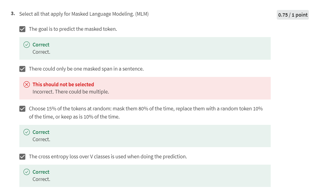
第三题正确答案：不选第二个，其他都选

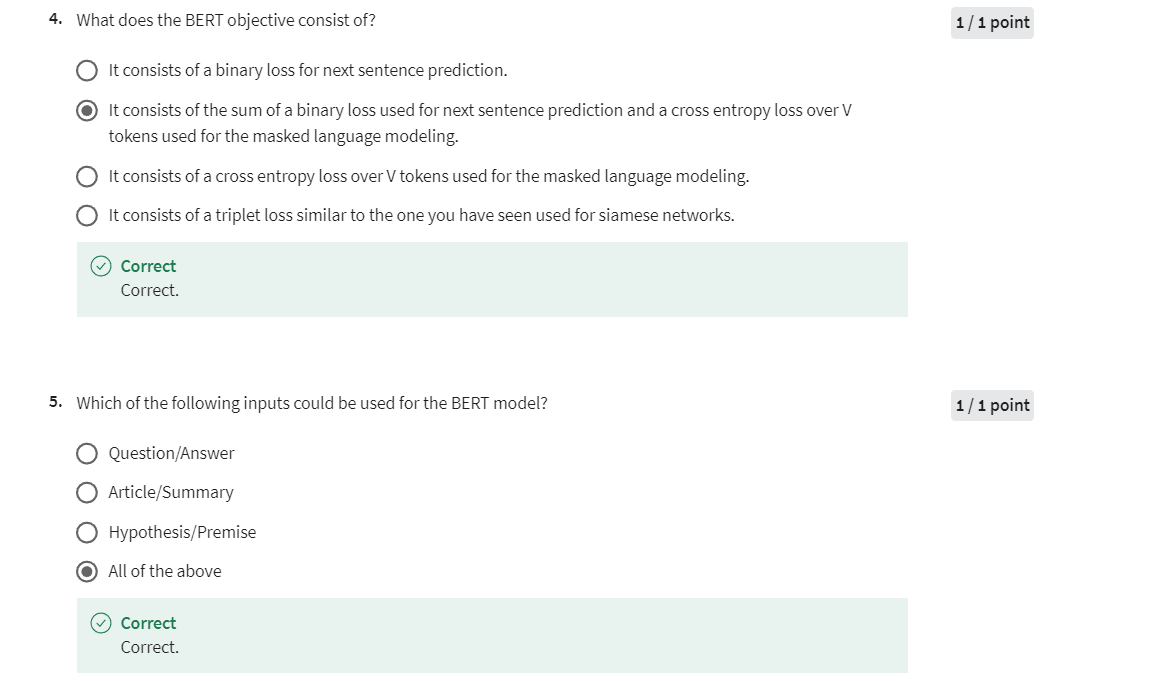
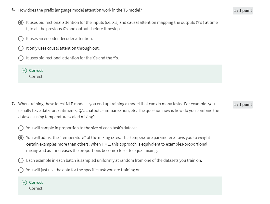
Programming Assignment: Question Answering

Assignment 3: Question Answering

Welcome to the third assignment of course 4. In this assignment you will explore question answering. You will implement the “Text to Text Transfer from Transformers” (better known as T5). Since you implemented transformers from scratch last week you will now be able to use them.

Overview

This assignment will be different from the two previous ones. Due to memory constraints of this environment and for the sake of time, your model will be trained with small datasets, so you won’t get models that you could use in production but you will gain the necessary knowledge about how the Generative Language models are trained and used. Also you won’t spend too much time with the architecture of the models but you will instead take a model that is pre-trained on a larger dataset and fine tune it to get better results.

After completing this labs you will:

• Understand how the C4 dataset is structured.
• Pretrain a transformer model using a Masked Language Model.
• Understand how the “Text to Text Transfer from Transformers” or T5 model works.
• Fine tune the T5 model for Question answering

Before getting started take some time to read the following tips:

TIPS FOR SUCCESSFUL GRADING OF YOUR ASSIGNMENT:

• All cells are frozen except for the ones where you need to submit your solutions.
• You can add new cells to experiment but these will be omitted by the grader, so don’t rely on newly created cells to host your solution code, use the provided places for this.
• You can add the comment # grade-up-to-here in any graded cell to signal the grader that it must only evaluate up to that point. This is helpful if you want to check if you are on the right track even if you are not done with the whole assignment. Be sure to remember to delete the comment afterwards!
• To submit your notebook, save it and then click on the blue submit button at the beginning of the page.

Importing the Packages

Let’s start by importing all the required libraries.

import os
os.environ['TF_CPP_MIN_LOG_LEVEL'] = '3'

import traceback
import time
import json
from termcolor import colored
import string
import textwrap
import itertools
import numpy as np
import tensorflow_text as tf_text
import tensorflow as tf

import transformer_utils 
import utils

# Will come in handy later
wrapper = textwrap.TextWrapper(width=70)

# Set random seed
np.random.seed(42)

import w3_unittest

1 - Prepare the data for pretraining T5

1.1 - Pre-Training Objective

In the initial phase of training a T5 model for a Question Answering task, the pre-training process involves leveraging a masked language model (MLM) on a very large dataset, such as the C4 dataset. The objective is to allow the model to learn contextualized representations of words and phrases, fostering a deeper understanding of language semantics. To initiate pre-training, it is essential to employ the Transformer architecture, which forms the backbone of T5. The Transformer’s self-attention mechanism enables the model to weigh different parts of the input sequence dynamically, capturing long-range dependencies effectively.

Before delving into pre-training, thorough data preprocessing is crucial. The C4 dataset, a diverse and extensive collection of web pages, provides a rich source for language understanding tasks. The dataset needs to be tokenized into smaller units, such as subwords or words, to facilitate model input. Additionally, the text is often segmented into fixed-length sequences or batches, optimizing computational efficiency during training.

For the masked language modeling objective, a percentage of the tokenized input is randomly masked, and the model is trained to predict the original content of these masked tokens. This process encourages the T5 model to grasp contextual relationships between words and phrases, enhancing its ability to generate coherent and contextually appropriate responses during downstream tasks like question answering.

In summary, the pre-training of the T5 model involves utilizing the Transformer architecture on a sizable dataset like C4, coupled with meticulous data preprocessing to convert raw text into a format suitable for training. The incorporation of a masked language modeling objective ensures that the model learns robust contextual representations, laying a solid foundation for subsequent fine-tuning on specific tasks such as question answering.

Note: The word “mask” will be used throughout this assignment in context of hiding/removing word(s)

You will be implementing the Masked language model (MLM) as shown in the following image.

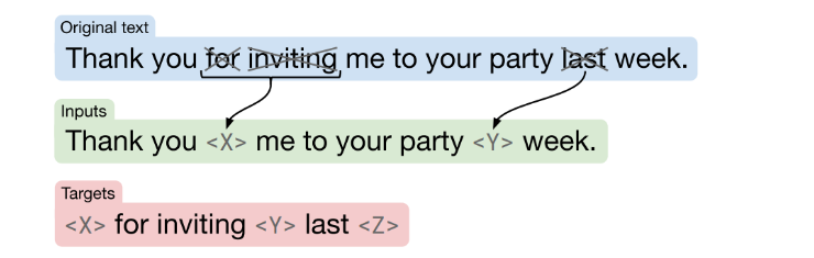
Assume you have the following text: Thank you for inviting me to your party last week

Now as input you will mask the words in red in the text:

Input: Thank you X me to your party Y week.

Output: The model should predict the words(s) for X and Y.

[EOS] will be used to mark the end of the target sequence.

1.2 - C4 Dataset

The C4 dataset, also known as the Common Crawl C4 (Common Crawl Corpus C4), is a large-scale dataset of web pages collected by the Common Crawl organization. It is commonly used for various natural language processing tasks and machine learning research. Each sample in the C4 dataset follows a consistent format, making it suitable for pretraining models like BERT. Here’s a short explanation and description of the C4 dataset:

• Format: Each sample in the C4 dataset is represented as a JSON object, containing several key-value pairs.

• Content: The ‘text’ field in each sample contains the actual text content extracted from web pages. This text often includes a wide range of topics and writing styles, making it diverse and suitable for training language models.

• Metadata: The dataset includes metadata such as ‘content-length,’ ‘content-type,’ ‘timestamp,’ and ‘url,’ providing additional information about each web page. ‘Content-length’ specifies the length of the content, ‘content-type’ describes the type of content (e.g., ‘text/plain’), ‘timestamp’ indicates when the web page was crawled, and ‘url’ provides the source URL of the web page.

• Applications: The C4 dataset is commonly used for training and fine-tuning large-scale language models, such as BERT. It serves as a valuable resource for tasks like text classification, named entity recognition, question answering, and more.

• Size: The C4 dataset is containing more than 800 GiB of text data, making it suitable for training models with billions of parameters.

Run the cell below to see how the C4 dataset looks like.

# Load example jsons
with open('data/c4-en-10k.jsonl', 'r') as file:
    example_jsons = [json.loads(line.strip()) for line in file]

# Printing the examples to see how the data looks like
for i in range(5):
    print(f'example number {i+1}: \n\n{example_jsons[i]} \n')

Output

example number 1: 

{'text': 'Beginners BBQ Class Taking Place in Missoula!\nDo you want to get better at making delicious BBQ? You will have the opportunity, put this on your calendar now. Thursday, September 22nd join World Class BBQ Champion, Tony Balay from Lonestar Smoke Rangers. He will be teaching a beginner level class for everyone who wants to get better with their culinary skills.\nHe will teach you everything you need to know to compete in a KCBS BBQ competition, including techniques, recipes, timelines, meat selection and trimming, plus smoker and fire information.\nThe cost to be in the class is $35 per person, and for spectators it is free. Included in the cost will be either a t-shirt or apron and you will be tasting samples of each meat that is prepared.'} 

example number 2: 

{'text': 'Discussion in \'Mac OS X Lion (10.7)\' started by axboi87, Jan 20, 2012.\nI\'ve got a 500gb internal drive and a 240gb SSD.\nWhen trying to restore using disk utility i\'m given the error "Not enough space on disk ____ to restore"\nBut I shouldn\'t have to do that!!!\nAny ideas or workarounds before resorting to the above?\nUse Carbon Copy Cloner to copy one drive to the other. I\'ve done this several times going from larger HDD to smaller SSD and I wound up with a bootable SSD drive. One step you have to remember not to skip is to use Disk Utility to partition the SSD as GUID partition scheme HFS+ before doing the clone. If it came Apple Partition Scheme, even if you let CCC do the clone, the resulting drive won\'t be bootable. CCC usually works in "file mode" and it can easily copy a larger drive (that\'s mostly empty) onto a smaller drive. If you tell CCC to clone a drive you did NOT boot from, it can work in block copy mode where the destination drive must be the same size or larger than the drive you are cloning from (if I recall).\nI\'ve actually done this somehow on Disk Utility several times (booting from a different drive (or even the dvd) so not running disk utility from the drive your cloning) and had it work just fine from larger to smaller bootable clone. Definitely format the drive cloning to first, as bootable Apple etc..\nThanks for pointing this out. My only experience using DU to go larger to smaller was when I was trying to make a Lion install stick and I was unable to restore InstallESD.dmg to a 4 GB USB stick but of course the reason that wouldn\'t fit is there was slightly more than 4 GB of data.'} 

example number 3: 

{'text': 'Foil plaid lycra and spandex shortall with metallic slinky insets. Attached metallic elastic belt with O-ring. Headband included. Great hip hop or jazz dance costume. Made in the USA.'} 

example number 4: 

{'text': "How many backlinks per day for new site?\nDiscussion in 'Black Hat SEO' started by Omoplata, Dec 3, 2010.\n1) for a newly created site, what's the max # backlinks per day I should do to be safe?\n2) how long do I have to let my site age before I can start making more blinks?\nI did about 6000 forum profiles every 24 hours for 10 days for one of my sites which had a brand new domain.\nThere is three backlinks for every of these forum profile so thats 18 000 backlinks every 24 hours and nothing happened in terms of being penalized or sandboxed. This is now maybe 3 months ago and the site is ranking on first page for a lot of my targeted keywords.\nbuild more you can in starting but do manual submission and not spammy type means manual + relevant to the post.. then after 1 month you can make a big blast..\nWow, dude, you built 18k backlinks a day on a brand new site? How quickly did you rank up? What kind of competition/searches did those keywords have?"} 

example number 5: 

{'text': 'The Denver Board of Education opened the 2017-18 school year with an update on projects that include new construction, upgrades, heat mitigation and quality learning environments.\nWe are excited that Denver students will be the beneficiaries of a four year, $572 million General Obligation Bond. Since the passage of the bond, our construction team has worked to schedule the projects over the four-year term of the bond.\nDenver voters on Tuesday approved bond and mill funding measures for students in Denver Public Schools, agreeing to invest $572 million in bond funding to build and improve schools and $56.6 million in operating dollars to support proven initiatives, such as early literacy.\nDenver voters say yes to bond and mill levy funding support for DPS students and schools. Click to learn more about the details of the voter-approved bond measure.\nDenver voters on Nov. 8 approved bond and mill funding measures for DPS students and schools. Learn more about what’s included in the mill levy measure.'} 

1.3 - Process C4

For the purpose of pretaining the T5 model, you will only use the content of each entry. In the following code, you filter only the field text from all the entries in the dataset. This is the data that you will use to create the inputs and targets of your language model.

# Grab text field from dictionary
natural_language_texts = [example_json['text'] for example_json in example_jsons]

# Print the first text example
print(natural_language_texts[0])

Output

Beginners BBQ Class Taking Place in Missoula!
Do you want to get better at making delicious BBQ? You will have the opportunity, put this on your calendar now. Thursday, September 22nd join World Class BBQ Champion, Tony Balay from Lonestar Smoke Rangers. He will be teaching a beginner level class for everyone who wants to get better with their culinary skills.
He will teach you everything you need to know to compete in a KCBS BBQ competition, including techniques, recipes, timelines, meat selection and trimming, plus smoker and fire information.
The cost to be in the class is $35 per person, and for spectators it is free. Included in the cost will be either a t-shirt or apron and you will be tasting samples of each meat that is prepared.

1.4 - Decode to Natural Language

The SentencePieceTokenizer, used in the code snippet, tokenizes text into subword units, enhancing handling of complex word structures, out-of-vocabulary words, and multilingual support. It simplifies preprocessing, ensures consistent tokenization, and seamlessly integrates with machine learning frameworks.

In this task, a SentencePiece model is loaded from a file, which is used to tokenize text into subwords represented by integer IDs.

# Special tokens
# PAD, EOS = 0, 1

with open("./models/sentencepiece.model", "rb") as f:
    pre_trained_tokenizer = f.read()
    
tokenizer = tf_text.SentencepieceTokenizer(pre_trained_tokenizer, out_type=tf.int32)

In this tokenizer the string </s> is used as EOS token. By default, the tokenizer does not add the EOS to the end of each sentence, so you need to add it manually when required. Let’s verify what id correspond to this token:

eos = tokenizer.string_to_id("</s>").numpy()

print("EOS: " + str(eos))

Output

EOS: 1

This code shows the process of tokenizing individual words from a given text, in this case, the first entry of the dataset.

# printing the encoding of each word to see how subwords are tokenized
tokenized_text = [(list(tokenizer.tokenize(word).numpy()), word) for word in natural_language_texts[2].split()]

print("Word\t\t-->\tTokenization")
print("-"*40)
for element in tokenized_text:
    print(f"{element[1]:<8}\t-->\t{element[0]}")

Output

Word		-->	Tokenization
----------------------------------------
Foil    	-->	[4452, 173]
plaid   	-->	[30772]
lycra   	-->	[3, 120, 2935]
and     	-->	[11]
spandex 	-->	[8438, 26, 994]
shortall	-->	[710, 1748]
with    	-->	[28]
metallic	-->	[18813]
slinky  	-->	[3, 7, 4907, 63]
insets. 	-->	[16, 2244, 7, 5]
Attached	-->	[28416, 15, 26]
metallic	-->	[18813]
elastic 	-->	[15855]
belt    	-->	[6782]
with    	-->	[28]
O-ring. 	-->	[411, 18, 1007, 5]
Headband	-->	[3642, 3348]
included.	-->	[1285, 5]
Great   	-->	[1651]
hip     	-->	[5436]
hop     	-->	[13652]
or      	-->	[42]
jazz    	-->	[9948]
dance   	-->	[2595]
costume.	-->	[11594, 5]
Made    	-->	[6465]
in      	-->	[16]
the     	-->	[8]
USA.    	-->	[2312, 5]

And as usual, the library provides a function to turn numeric tokens into human readable text. Look how it works.

# We can see that detokenize successfully undoes the tokenization
print(f"tokenized: {tokenizer.tokenize('Beginners')}\ndetokenized: {tokenizer.detokenize(tokenizer.tokenize('Beginners'))}")

Output

tokenized: [12847   277]
detokenized: b'Beginners'

As you can see above, you were able to take a piece of string and tokenize it.

Now you will create input and target pairs that will allow you to train your model. T5 uses the ids at the end of the vocab file as sentinels. For example, it will replace:

• vocab_size - 1 by <Z>
• vocab_size - 2 by <Y>
• and so forth.

It assigns every word a chr.

The pretty_decode function below, which you will use in a bit, helps in handling the type when decoding. Take a look and try to understand what the function is doing.

Notice that:

string.ascii_letters = 'abcdefghijklmnopqrstuvwxyzABCDEFGHIJKLMNOPQRSTUVWXYZ'

NOTE: Targets may have more than the 52 sentinels we replace, but this is just to give you an idea of things.

def get_sentinels(tokenizer, display=False):
    sentinels = {}
    vocab_size = tokenizer.vocab_size(name=None)
    for i, char in enumerate(reversed(string.ascii_letters), 1):
        decoded_text = tokenizer.detokenize([vocab_size - i]).numpy().decode("utf-8")
        
        # Sentinels, ex: <Z> - <a>
        sentinels[decoded_text] = f'<{char}>'    
    
        if display:
            print(f'The sentinel is <{char}> and the decoded token is:', decoded_text)

    return sentinels

def pretty_decode(encoded_str_list, sentinels, tokenizer):
    # If already a string, just do the replacements.
    if tf.is_tensor(encoded_str_list) and encoded_str_list.dtype == tf.string:
        for token, char in sentinels.items():
            encoded_str_list = tf.strings.regex_replace(encoded_str_list, token, char)
        return encoded_str_list
  
    # We need to decode and then prettyfy it.
    return pretty_decode(tokenizer.detokenize(encoded_str_list), sentinels, tokenizer)

sentinels = get_sentinels(tokenizer, display=True)

Output

The sentinel is <Z> and the decoded token is: Internațional
The sentinel is <Y> and the decoded token is: erwachsene
The sentinel is <X> and the decoded token is: Cushion
The sentinel is <W> and the decoded token is: imunitar
The sentinel is <V> and the decoded token is: Intellectual
The sentinel is <U> and the decoded token is: traditi
The sentinel is <T> and the decoded token is: disguise
The sentinel is <S> and the decoded token is: exerce
The sentinel is <R> and the decoded token is: nourishe
The sentinel is <Q> and the decoded token is: predominant
The sentinel is <P> and the decoded token is: amitié
The sentinel is <O> and the decoded token is: erkennt
The sentinel is <N> and the decoded token is: dimension
The sentinel is <M> and the decoded token is: inférieur
The sentinel is <L> and the decoded token is: refugi
The sentinel is <K> and the decoded token is: cheddar
The sentinel is <J> and the decoded token is: unterlieg
The sentinel is <I> and the decoded token is: garanteaz
The sentinel is <H> and the decoded token is: făcute
The sentinel is <G> and the decoded token is: réglage
The sentinel is <F> and the decoded token is: pedepse
The sentinel is <E> and the decoded token is: Germain
The sentinel is <D> and the decoded token is: distinctly
The sentinel is <C> and the decoded token is: Schraub
The sentinel is <B> and the decoded token is: emanat
The sentinel is <A> and the decoded token is: trimestre
The sentinel is <z> and the decoded token is: disrespect
The sentinel is <y> and the decoded token is: Erasmus
The sentinel is <x> and the decoded token is: Australia
The sentinel is <w> and the decoded token is: permeabil
The sentinel is <v> and the decoded token is: deseori
The sentinel is <u> and the decoded token is: manipulated
The sentinel is <t> and the decoded token is: suggér
The sentinel is <s> and the decoded token is: corespund
The sentinel is <r> and the decoded token is: nitro
The sentinel is <q> and the decoded token is: oyons
The sentinel is <p> and the decoded token is: Account
The sentinel is <o> and the decoded token is: échéan
The sentinel is <n> and the decoded token is: laundering
The sentinel is <m> and the decoded token is: genealogy
The sentinel is <l> and the decoded token is: QuickBooks
The sentinel is <k> and the decoded token is: constituted
The sentinel is <j> and the decoded token is: Fertigung
The sentinel is <i> and the decoded token is: goutte
The sentinel is <h> and the decoded token is: regulă
The sentinel is <g> and the decoded token is: overwhelmingly
The sentinel is <f> and the decoded token is: émerg
The sentinel is <e> and the decoded token is: broyeur
The sentinel is <d> and the decoded token is: povești
The sentinel is <c> and the decoded token is: emulator
The sentinel is <b> and the decoded token is: halloween
The sentinel is <a> and the decoded token is: combustibil

Now, let’s use the pretty_decode function in the following sentence. Note that all the words listed as sentinels, will be replaced by the function with the corresponding sentinel. It could be a drawback of this method, but don’t worry about it now.

pretty_decode(tf.constant("I want to dress up as an Intellectual this halloween."), sentinels, tokenizer)

Output

<tf.Tensor: shape=(), dtype=string, numpy=b'I want to dress up as an <V> this <b>.'>

The functions above make your inputs and targets more readable. For example, you might see something like this once you implement the masking function below.

• Input sentence: Younes and Lukasz were working together in the lab yesterday after lunch.
• Input: Younes and Lukasz Z together in the Y yesterday after lunch.
• Target: Z were working Y lab.

1.5 - Tokenizing and Masking

In this task, you will implement the tokenize_and_mask function, which tokenizes and masks input words based on a given probability. The probability is controlled by the noise parameter, typically set to mask around 15% of the words in the input text. The function will generate two lists of tokenized sequences following the algorithm outlined below:

Exercise 1 - tokenize_and_mask

• Start with two empty lists: inps and targs
• Tokenize the input text using the given tokenizer.
• For each token in the tokenized sequence:
  • Generate a random number(simulating a weighted coin toss)
  • If the random value is greater than the given threshold(noise):
    • Add the current token to the inps list
  • Else:
    • If a new sentinel must be included(read note **):
      • Compute the next sentinel ID using a progression.
      • Add a sentinel into the inps and targs to mark the position of the masked element.
    • Add the current token to the targs list.

** There’s a special case to consider. If two or more consecutive tokens get masked during the process, you don’t need to add a new sentinel to the sequences. To account for this, use the prev_no_mask flag, which starts as True but is turned to False each time you mask a new element. The code that adds sentinels will only be executed if, before masking the token, the flag was in the True state.

# GRADED FUNCTION: tokenize_and_mask
def tokenize_and_mask(text, 
                      noise=0.15, 
                      randomizer=np.random.uniform, 
                      tokenizer=None):
    """Tokenizes and masks a given input.

    Args:
        text (str or bytes): Text input.
        noise (float, optional): Probability of masking a token. Defaults to 0.15.
        randomizer (function, optional): Function that generates random values. Defaults to np.random.uniform.
        tokenizer (function, optional): Tokenizer function. Defaults to tokenize.

    Returns:
        inps, targs: Lists of integers associated to inputs and targets.
    """
    
    # Current sentinel number (starts at 0)
    cur_sentinel_num = 0
    
    # Inputs and targets
    inps, targs = [], []

    # Vocab_size
    vocab_size = int(tokenizer.vocab_size())
    
    # EOS token id 
    # Must be at the end of each target!
    eos = tokenizer.string_to_id("</s>").numpy()
    
    ### START CODE HERE ###
    
    # prev_no_mask is True if the previous token was NOT masked, False otherwise
    # set prev_no_mask to True
    prev_no_mask = True
    
    # Loop over the tokenized text
    for token in tokenizer.tokenize(text).numpy():
        
        # Generate a random value between 0 and 1
        rnd_val = randomizer() 
        
        # Check if the noise is greater than a random value (weighted coin flip)
        if noise > rnd_val:
            
            # Check if previous token was NOT masked
            if prev_no_mask:
                
                # Current sentinel increases by 1
                cur_sentinel_num += 1
                
                # Compute end_id by subtracting current sentinel value out of the total vocabulary size
                end_id = vocab_size - cur_sentinel_num
                
                # Append end_id at the end of the targets
                targs.append(end_id)
                
                # Append end_id at the end of the inputs
                inps.append(end_id)
                
            # Append token at the end of the targets
            targs.append(token)
            
            # set prev_no_mask accordingly
            prev_no_mask = False

        else:
            
            # Append token at the end of the inputs
            inps.append(token)
            
            # Set prev_no_mask accordingly
            prev_no_mask = True
    
    
    # Add EOS token to the end of the targets
    targs.append(eos)
    
    ### END CODE HERE ###
    
    return inps, targs

# Some logic to mock a np.random value generator
# Needs to be in the same cell for it to always generate same output
def testing_rnd():
    def dummy_generator():
        vals = np.linspace(0, 1, 10)
        cyclic_vals = itertools.cycle(vals)
        for _ in range(100):
            yield next(cyclic_vals)

    dumr = itertools.cycle(dummy_generator())

    def dummy_randomizer():
        return next(dumr)
    
    return dummy_randomizer

input_str = 'Beginners BBQ Class Taking Place in Missoula!\nDo you want to get better at making delicious BBQ? You will have the opportunity, put this on your calendar now. Thursday, September 22nd join World Class BBQ Champion, Tony Balay from Lonestar Smoke Rangers.'

inps, targs = tokenize_and_mask(input_str, randomizer=testing_rnd(), tokenizer=tokenizer)
print(f"tokenized inputs - shape={len(inps)}:\n\n{inps}\n\ntargets - shape={len(targs)}:\n\n{targs}")

Output

tokenized inputs - shape=53:

[31999, 15068, 4501, 3, 12297, 3399, 16, 5964, 7115, 31998, 531, 25, 241, 12, 129, 394, 44, 492, 31997, 58, 148, 56, 43, 8, 1004, 6, 474, 31996, 39, 4793, 230, 5, 2721, 6, 1600, 1630, 31995, 1150, 4501, 15068, 16127, 6, 9137, 2659, 5595, 31994, 782, 3624, 14627, 15, 12612, 277, 5]

targets - shape=19:

[31999, 12847, 277, 31998, 9, 55, 31997, 3326, 15068, 31996, 48, 30, 31995, 727, 1715, 31994, 45, 301, 1]

Expected Output:

tokenized inputs - shape=53:

[31999 15068  4501     3 12297  3399    16  5964  7115 31998   531    25
   241    12   129   394    44   492 31997    58   148    56    43     8
  1004     6   474 31996    39  4793   230     5  2721     6  1600  1630
 31995  1150  4501 15068 16127     6  9137  2659  5595 31994   782  3624
 14627    15 12612   277     5]

targets - shape=19:

[31999 12847   277 31998     9    55 31997  3326 15068 31996    48    30
 31995   727  1715 31994    45   301     1]

# Test your implementation!
w3_unittest.test_tokenize_and_mask(tokenize_and_mask)

Output

 All tests passed

You will now use the inputs and the targets from the tokenize_and_mask function you implemented above. Take a look at the decoded version of your masked sentence using your inps and targs from the sentence above.

print('Inputs: \n\n', pretty_decode(inps, sentinels, tokenizer).numpy())
print('\nTargets: \n\n', pretty_decode(targs, sentinels, tokenizer).numpy())

Output

Inputs: 

 b'<Z> BBQ Class Taking Place in Missoul <Y> Do you want to get better at making <X>? You will have the opportunity, put <W> your calendar now. Thursday, September 22 <V> World Class BBQ Champion, Tony Balay <U>onestar Smoke Rangers.'

Targets: 

 b'<Z> Beginners <Y>a! <X> delicious BBQ <W> this on <V>nd join <U> from L'

1.6 - Creating the Pairs

You will now create pairs using your dataset. You will iterate over your data and create (inp, targ) pairs using the functions that we have given you.

# Apply tokenize_and_mask
inputs_targets_pairs = [tokenize_and_mask(text.encode('utf-8', errors='ignore').decode('utf-8'), tokenizer=tokenizer) 
                        for text in natural_language_texts[0:2000]]

def display_input_target_pairs(inputs_targets_pairs, sentinels, wrapper=textwrap.TextWrapper(width=70), tokenizer=tokenizer):
    for i, inp_tgt_pair in enumerate(inputs_targets_pairs, 1):
        inps, tgts = inp_tgt_pair
        inps = str(pretty_decode(inps, sentinels, tokenizer).numpy(), encoding='utf-8')
        tgts = str(pretty_decode(tgts, sentinels, tokenizer).numpy(), encoding='utf-8')
        print(f'[{i}]\n\n'
              f'inputs:\n{wrapper.fill(text=inps)}\n\n'
              f'targets:\n{wrapper.fill(text=tgts)}\n\n\n')

# Print 3 samples. We print inputs with less than 100 tokens. It is just to give you and idea of the process
display_input_target_pairs(filter(lambda x: len(x[0]) < 100, inputs_targets_pairs[0:12]), sentinels, wrapper, tokenizer)

Output

[1]

inputs:
<Z>il plaid <Y>lycra <X> spandex shortall with metallic slinky
<W>sets. Attache <V> metallic elastic belt with O <U>ring. Head <T>
included. Great hip hop<S> jazz dance costume.<R> in the USA.

targets:
<Z> Fo <Y>  <X> and <W> in <V>d <U>- <T>band<S> or<R> Made



[2]

inputs:
I thought I was going to <Z> 3rd season <Y> Wire tonight. <X> there
was a commentary <W> 11, so I had to re <V>watch <U> Ground with <T>
commentary. Hopefully<S> can finish<R> season <Q>.

targets:
<Z> finish the <Y> of the <X> But <W> on episode <V>- <U> Middle <T>
the<S> I<R> the <Q> next weekend



[3]

inputs:
Pencarian <Z>FILM Untuk " <Y>eace <X>er 2017 <W> yuk mampir ke channel
say <V>. Edges <U> provides the l.. A corrupt cop makes one w.. <T>er
2017  ⁇ <S> ⁇  .. Náo Lo ⁇ n - Peace Break.. Please subscribe and hit
..<R> in HD at http://.. <Q> cannot believe I manage..

targets:
<Z>  <Y>P <X> Break <W>" <V>. <U> East <T> Peace Break<S> <R> uploaded
<Q> I

2 - Pretrain a T5 model using C4

Now you are going to use the Transformer’s architecture that you coded in the previous assignment to summarize text, but this time to answer questions. Instead of training the question answering model from scratch, you will first “pre-train” the model using the C4 data set you just processed. This will help the model to learn the general structure of language from a large dataset. This is much easier to do, as you don’t need to label any data, but just use the masking, which is done automatically. You will then use the data from the SQuAD set to teach the model to answer questions given a context. To start let’s review the Transformer’s architecture.

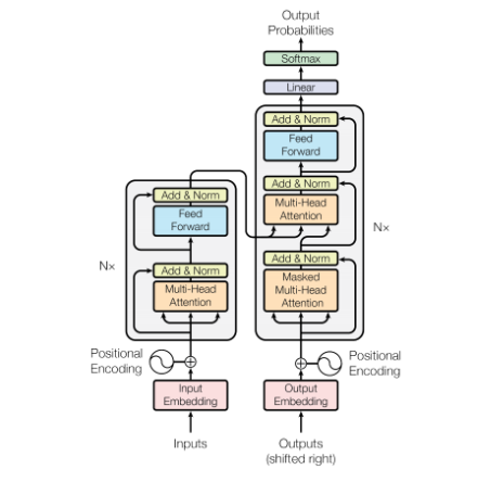
2.1 - Instantiate a new transformer model

We have packaged the code implemented in the previous week into the Transformer.py file. You can import it here, and setup with the same configuration used there.

transformer_utils.py文件的内容和这门课的week2实现的Transformer一样，请参加Week2的笔记。

# Define the model parameters
num_layers = 2
embedding_dim = 128
fully_connected_dim = 128
num_heads = 2
positional_encoding_length = 256

encoder_vocab_size = int(tokenizer.vocab_size())
decoder_vocab_size = encoder_vocab_size

# Initialize the model
transformer = transformer_utils.Transformer(
    num_layers, 
    embedding_dim, 
    num_heads, 
    fully_connected_dim,
    encoder_vocab_size, 
    decoder_vocab_size, 
    positional_encoding_length, 
    positional_encoding_length,
)

Now, you will define the optimizer and the loss function. For this task the model will try to predict the masked words, so, as in the previous lab, the loss function will be the SparseCategoricalCrossEntropy.

learning_rate = transformer_utils.CustomSchedule(embedding_dim)
optimizer = tf.keras.optimizers.Adam(0.0001, beta_1=0.9, beta_2=0.98, epsilon=1e-9)

loss_object = tf.keras.losses.SparseCategoricalCrossentropy(from_logits=True, reduction='none')
train_loss = tf.keras.metrics.Mean(name='train_loss')

# Here you will store the losses, so you can later plot them
losses = []

2.2 - C4 pretraining

For training a Tensorflow model you need to arrange the data into datasets. Now, you will get the inputs and the targets for the transformer model from the inputs_targets_pairs. Before creating the dataset, you need to be sure that all inputs have the same length by truncating the longer sequences and padding the shorter ones with 0. The same must be done for the targets. The function tf.keras.preprocessing.sequence.pad_sequences will help you here, as in the previous week assignment.

You will use a BATCH_SIZE = 64

# Limit the size of the input and output data so this can run in this environment
encoder_maxlen = 150
decoder_maxlen = 50

inputs = tf.keras.preprocessing.sequence.pad_sequences([x[0] for x in inputs_targets_pairs], maxlen=encoder_maxlen, padding='post', truncating='post')
targets = tf.keras.preprocessing.sequence.pad_sequences([x[1] for x in inputs_targets_pairs], maxlen=decoder_maxlen, padding='post', truncating='post')

inputs = tf.cast(inputs, dtype=tf.int32)
targets = tf.cast(targets, dtype=tf.int32)

# Create the final training dataset.
BUFFER_SIZE = 10000
BATCH_SIZE = 64

dataset = tf.data.Dataset.from_tensor_slices((inputs, targets)).shuffle(BUFFER_SIZE).batch(BATCH_SIZE)

Now, you can run the training loop for 10 epochs. Running it with a big dataset such as C4 on a good computer with enough memory and a good GPU could take more than 24 hours. Here, you will run few epochs using a small portion of the C4 dataset for illustration. It will only take a few minutes, but the model won’t be very powerful.

# Define the number of epochs
epochs = 10

# Training loop
for epoch in range(epochs):
    
    start = time.time()
    train_loss.reset_states()
    number_of_batches=len(list(enumerate(dataset)))

    for (batch, (inp, tar)) in enumerate(dataset):
        print(f'Epoch {epoch+1}, Batch {batch+1}/{number_of_batches}', end='\r')
        transformer_utils.train_step(inp, tar, transformer, loss_object, optimizer, train_loss)
    
    print (f'Epoch {epoch+1}, Loss {train_loss.result():.4f}')
    losses.append(train_loss.result())
    
    print (f'Time taken for one epoch: {time.time() - start} sec')

# Save the pretrained model
# transformer.save_weights('./model_c4_temp')

Output

Epoch 1, Loss 10.1099
Time taken for one epoch: 27.699499130249023 sec
Epoch 2, Loss 9.5039
Time taken for one epoch: 9.490442514419556 sec
Epoch 3, Loss 8.9165
Time taken for one epoch: 7.633259534835815 sec
Epoch 4, Loss 8.3763
Time taken for one epoch: 6.909319877624512 sec
Epoch 5, Loss 7.8829
Time taken for one epoch: 6.5587158203125 sec
Epoch 6, Loss 7.4371
Time taken for one epoch: 4.343854188919067 sec
Epoch 7, Loss 7.0420
Time taken for one epoch: 5.894981861114502 sec
Epoch 8, Loss 6.7049
Time taken for one epoch: 4.371525287628174 sec
Epoch 9, Loss 6.4366
Time taken for one epoch: 3.7441866397857666 sec
Epoch 10, Loss 6.2313
Time taken for one epoch: 4.185030937194824 sec

Load a pretrained model

To show how powerful this model actually is, we trained it for several epochs with the full dataset in Colab and saved the weights for you. You can load them using the cell below. For the rest of the notebook, you will see the power of the transfer learning in action.

transformer.load_weights('./pretrained_models/model_c4')

3. Fine tune the T5 model for Question Answering

Now, you are going to fine tune the pretrained model for Question Answering using the SQUad 2.0 dataset.

SQuAD, short for Stanford Question Answering Dataset, is a dataset designed for training and evaluating question answering systems. It consists of real questions posed by humans on a set of Wikipedia articles, where the answer to each question is a specific span of text within the corresponding article.

SQuAD 1.1, the previous version of the SQuAD dataset, contains 100,000+ question-answer pairs on about 500 articles.
SQuAD 2.0, contains 50.000 additional questions that are not meant to be answered. This extra set of questions can help to train models to detect unanswerable questions.

Let’s load the dataset.

with open('data/train-v2.0.json', 'r') as f:
    example_jsons = json.load(f)

example_jsons = example_jsons['data']

print('Number of articles: ' + str(len(example_jsons)))

Output

Number of articles: 442

The structure of each article is as follows:

• title: The article title
• paragraphs: A list of paragraphs and questions related to them
  • context: The actual paragraph text
  • qas: A set of question related to the paragraph
    • question: A question
    • id: The question unique identifier
    • is_imposible: Boolean, specifies if the question can be answered or not
    • answers: A set of possible answers for the question
      • text: The answer
      • answer_start: The index of the character that starts the sentence containing the explicit answer to the question

Take a look at an article by running the next cell. Notice that the context is usually the last element for every paragraph:

example_article = example_jsons[0]
example_article

print("Title: " + example_article["title"])
print(example_article["paragraphs"][0])

Output

Title: Beyoncé
{'qas': [{'question': 'When did Beyonce start becoming popular?', 'id': '56be85543aeaaa14008c9063', 'answers': [{'text': 'in the late 1990s', 'answer_start': 269}], 'is_impossible': False}, {'question': 'What areas did Beyonce compete in when she was growing up?', 'id': '56be85543aeaaa14008c9065', 'answers': [{'text': 'singing and dancing', 'answer_start': 207}], 'is_impossible': False}, {'question': "When did Beyonce leave Destiny's Child and become a solo singer?", 'id': '56be85543aeaaa14008c9066', 'answers': [{'text': '2003', 'answer_start': 526}], 'is_impossible': False}, {'question': 'In what city and state did Beyonce  grow up? ', 'id': '56bf6b0f3aeaaa14008c9601', 'answers': [{'text': 'Houston, Texas', 'answer_start': 166}], 'is_impossible': False}, {'question': 'In which decade did Beyonce become famous?', 'id': '56bf6b0f3aeaaa14008c9602', 'answers': [{'text': 'late 1990s', 'answer_start': 276}], 'is_impossible': False}, {'question': 'In what R&B group was she the lead singer?', 'id': '56bf6b0f3aeaaa14008c9603', 'answers': [{'text': "Destiny's Child", 'answer_start': 320}], 'is_impossible': False}, {'question': 'What album made her a worldwide known artist?', 'id': '56bf6b0f3aeaaa14008c9604', 'answers': [{'text': 'Dangerously in Love', 'answer_start': 505}], 'is_impossible': False}, {'question': "Who managed the Destiny's Child group?", 'id': '56bf6b0f3aeaaa14008c9605', 'answers': [{'text': 'Mathew Knowles', 'answer_start': 360}], 'is_impossible': False}, {'question': 'When did Beyoncé rise to fame?', 'id': '56d43c5f2ccc5a1400d830a9', 'answers': [{'text': 'late 1990s', 'answer_start': 276}], 'is_impossible': False}, {'question': "What role did Beyoncé have in Destiny's Child?", 'id': '56d43c5f2ccc5a1400d830aa', 'answers': [{'text': 'lead singer', 'answer_start': 290}], 'is_impossible': False}, {'question': 'What was the first album Beyoncé released as a solo artist?', 'id': '56d43c5f2ccc5a1400d830ab', 'answers': [{'text': 'Dangerously in Love', 'answer_start': 505}], 'is_impossible': False}, {'question': 'When did Beyoncé release Dangerously in Love?', 'id': '56d43c5f2ccc5a1400d830ac', 'answers': [{'text': '2003', 'answer_start': 526}], 'is_impossible': False}, {'question': 'How many Grammy awards did Beyoncé win for her first solo album?', 'id': '56d43c5f2ccc5a1400d830ad', 'answers': [{'text': 'five', 'answer_start': 590}], 'is_impossible': False}, {'question': "What was Beyoncé's role in Destiny's Child?", 'id': '56d43ce42ccc5a1400d830b4', 'answers': [{'text': 'lead singer', 'answer_start': 290}], 'is_impossible': False}, {'question': "What was the name of Beyoncé's first solo album?", 'id': '56d43ce42ccc5a1400d830b5', 'answers': [{'text': 'Dangerously in Love', 'answer_start': 505}], 'is_impossible': False}], 'context': 'Beyoncé Giselle Knowles-Carter (/biːˈjɒnseɪ/ bee-YON-say) (born September 4, 1981) is an American singer, songwriter, record producer and actress. Born and raised in Houston, Texas, she performed in various singing and dancing competitions as a child, and rose to fame in the late 1990s as lead singer of R&B girl-group Destiny\'s Child. Managed by her father, Mathew Knowles, the group became one of the world\'s best-selling girl groups of all time. Their hiatus saw the release of Beyoncé\'s debut album, Dangerously in Love (2003), which established her as a solo artist worldwide, earned five Grammy Awards and featured the Billboard Hot 100 number-one singles "Crazy in Love" and "Baby Boy".'}

The previous article might be difficult to navigate so here is a nicely formatted example paragraph:

{
  "context": "Beyoncé Giselle Knowles-Carter (/biːˈjɒnseɪ/ bee-YON-say) (born September 4, 1981) is an American singer, songwriter, record producer and actress. Born and raised in Houston, Texas, she performed in various singing and dancing competitions as a child, and rose to fame in the late 1990s as lead singer of R&B girl-group Destiny's Child. Managed by her father, Mathew Knowles, the group became one of the world's best-selling girl groups of all time. Their hiatus saw the release of Beyoncé's debut album, Dangerously in Love (2003), which established her as a solo artist worldwide, earned five Grammy Awards and featured the Billboard Hot 100 number-one singles 'Crazy in Love' and 'Baby Boy'",
  "qas": [
    {
      "question": "When did Beyonce start becoming popular?",
      "id": "56be85543aeaaa14008c9063",
      "answers": [
        {
          "text": "in the late 1990s",
          "answer_start": 269
        }
      ],
      "is_impossible": false
    },
    {
      "question": "What areas did Beyonce compete in when she was growing up?",
      "id": "56be85543aeaaa14008c9065",
      "answers": [
        {
          "text": "singing and dancing",
          "answer_start": 207
        }
      ],
      "is_impossible": false
    }
  ]
}

3.1 - Creating a list of paired question and answers

You are tasked with generating input/output pairs for a Question Answering (QA) model using the SQuAD 2.0 dataset. Each pair follows the structure:

• inputs: question: <Q> context: <P>
• targets: answer: <A>

Here, <Q> represents the question in the context of the given paragraph <P>, and <A> is a possible answer.

In this notebook, we will focus on a single answer per question. However, it’s essential to note that the dataset contains questions with multiple answers. When training a model in real-life scenarios, consider including all available information.

Exercise 2 - Parse the SQuaD 2.0 Dataset

Your task is to implement the parse_squad function, which iterates over all the articles, paragraphs, and questions in the SQuAD dataset. Extract pairs of inputs and targets for the QA model using the provided code template.

• Start with two empty lists: inputs and targets.
• Loop over all the articles in the dataset.
• For each article, loop over each paragraph.
• Extract the context from the paragraph.
• Loop over each question in the given paragraph.
• Check if the question is not impossible and has at least one answer.
• If the above condition is met, create the question_context sequence as described in the input structure.
• Create the answer sequence using the first answer from the available answers.
• Append the question_context to the inputs list.
• Append the answer to the targets list.

# GRADED FUNCTION: parse_squad
def parse_squad(dataset):
    """Extract all the answers/questions pairs from the SQuAD dataset

    Args:
        dataset (dict): The imported JSON dataset

    Returns:
        inputs, targets: Two lists containing the inputs and the targets for the QA model
    """

    inputs, targets = [], []

    ### START CODE HERE ###
    
    # Loop over all the articles
    for article in dataset:
        
        # Loop over each paragraph of each article
        for paragraph in article["paragraphs"]:
            
            # Extract context from the paragraph
            context = paragraph["context"]
            
            #Loop over each question of the given paragraph
            for qa in paragraph["qas"]:
                
                # If this question is not impossible and there is at least one answer
                if len(qa['answers']) > 0 and not(qa['is_impossible']):
                    
                    # Create the question/context sequence
                    question_context = 'question: ' + qa["question"] + ' context: ' + context
                    
                    # Create the answer sequence. Use the text field of the first answer
                    answer = 'answer: ' + qa["answers"][0]["text"]
                    
                    # Add the question_context to the inputs list
                    inputs.append(question_context)
                    
                    # Add the answer to the targets list
                    targets.append(answer)
    
    ### END CODE HERE ###
    
    return inputs, targets

inputs, targets =  parse_squad(example_jsons)          
print("Number of question/answer pairs: " + str(len(inputs)))

print('\nFirst Q/A pair:\n\ninputs: ' + colored(inputs[0], 'blue'))
print('\ntargets: ' + colored(targets[0], 'green'))
print('\nLast Q/A pair:\n\ninputs: ' + colored(inputs[-1], 'blue'))
print('\ntargets: ' + colored(targets[-1], 'green'))

Output

Number of question/answer pairs: 86821

First Q/A pair:

inputs: question: When did Beyonce start becoming popular? context: Beyoncé Giselle Knowles-Carter (/biːˈjɒnseɪ/ bee-YON-say) (born September 4, 1981) is an American singer, songwriter, record producer and actress. Born and raised in Houston, Texas, she performed in various singing and dancing competitions as a child, and rose to fame in the late 1990s as lead singer of R&B girl-group Destiny's Child. Managed by her father, Mathew Knowles, the group became one of the world's best-selling girl groups of all time. Their hiatus saw the release of Beyoncé's debut album, Dangerously in Love (2003), which established her as a solo artist worldwide, earned five Grammy Awards and featured the Billboard Hot 100 number-one singles "Crazy in Love" and "Baby Boy".

targets: answer: in the late 1990s

Last Q/A pair:

inputs: question: What is KMC an initialism of? context: Kathmandu Metropolitan City (KMC), in order to promote international relations has established an International Relations Secretariat (IRC). KMC's first international relationship was established in 1975 with the city of Eugene, Oregon, United States. This activity has been further enhanced by establishing formal relationships with 8 other cities: Motsumoto City of Japan, Rochester of the USA, Yangon (formerly Rangoon) of Myanmar, Xi'an of the People's Republic of China, Minsk of Belarus, and Pyongyang of the Democratic Republic of Korea. KMC's constant endeavor is to enhance its interaction with SAARC countries, other International agencies and many other major cities of the world to achieve better urban management and developmental programs for Kathmandu.

targets: answer: Kathmandu Metropolitan City

Expected Output:

Number of question/answer pairs: 86821

First Q/A pair:

inputs: question: When did Beyonce start becoming popular? context: Beyoncé Giselle Knowles-Carter (/biːˈjɒnseɪ/ bee-YON-say) (born September 4, 1981) is an American singer, songwriter, record producer and actress. Born and raised in Houston, Texas, she performed in various singing and dancing competitions as a child, and rose to fame in the late 1990s as lead singer of R&B girl-group Destiny's Child. Managed by her father, Mathew Knowles, the group became one of the world's best-selling girl groups of all time. Their hiatus saw the release of Beyoncé's debut album, Dangerously in Love (2003), which established her as a solo artist worldwide, earned five Grammy Awards and featured the Billboard Hot 100 number-one singles "Crazy in Love" and "Baby Boy".

targets: answer: in the late 1990s

Last Q/A pair:

inputs: question: What is KMC an initialism of? context: Kathmandu Metropolitan City (KMC), in order to promote international relations has established an International Relations Secretariat (IRC). KMC's first international relationship was established in 1975 with the city of Eugene, Oregon, United States. This activity has been further enhanced by establishing formal relationships with 8 other cities: Motsumoto City of Japan, Rochester of the USA, Yangon (formerly Rangoon) of Myanmar, Xi'an of the People's Republic of China, Minsk of Belarus, and Pyongyang of the Democratic Republic of Korea. KMC's constant endeavor is to enhance its interaction with SAARC countries, other International agencies and many other major cities of the world to achieve better urban management and developmental programs for Kathmandu.

targets: answer: Kathmandu Metropolitan City

# UNIT TEST
w3_unittest.test_parse_squad(parse_squad)

Output

All tests passed

You will use 40000 samples for training and 5000 samples for testing

# 40K pairs for training
inputs_train = inputs[0:40000] 
targets_train = targets[0:40000]  

# 5K pairs for testing
inputs_test = inputs[40000:45000] 
targets_test =  targets[40000:45000] 

Now, you can create the batch dataset of padded sequences. You will first tokenize the inputs and the targets. Then, using the function tf.keras.preprocessing.sequence.pad_sequences, you will ensure that the inputs and the outputs have the required lengths. Remember that the sequences longer than the required size will be truncated and the shorter ones will be padded with 0. This setup is very similar to the other one used in this and the previous notebook.

# Limit the size of the input and output data so this can run in this environment
encoder_maxlen = 150
decoder_maxlen = 50

inputs_str = [tokenizer.tokenize(s) for s in inputs_train]
targets_str = [tf.concat([tokenizer.tokenize(s), [1]], 0) for s in targets_train]

inputs = tf.keras.preprocessing.sequence.pad_sequences(inputs_str, maxlen=encoder_maxlen, padding='post', truncating='post')
targets = tf.keras.preprocessing.sequence.pad_sequences(targets_str, maxlen=decoder_maxlen, padding='post', truncating='post')

inputs = tf.cast(inputs, dtype=tf.int32)
targets = tf.cast(targets, dtype=tf.int32)

# Create the final training dataset.
BUFFER_SIZE = 10000
BATCH_SIZE = 64
dataset = tf.data.Dataset.from_tensor_slices((inputs, targets)).shuffle(BUFFER_SIZE).batch(BATCH_SIZE)

3.2 Fine tune the T5 model

Now, you will train the model for 2 epochs. In the T5 model, all the weights are adjusted during the fine tuning. As usual, fine tuning this model to get state of the art results would require more time and resources than there are available in this environment, but you are welcome to train the model for more epochs and with more data using Colab GPUs.

# Define the number of epochs
epochs = 2
losses = []

# Training loop
for epoch in range(epochs):
    
    start = time.time()
    train_loss.reset_states()
    number_of_batches=len(list(enumerate(dataset)))

    for (batch, (inp, tar)) in enumerate(dataset):
        print(f'Epoch {epoch+1}, Batch {batch+1}/{number_of_batches}', end='\r')
        transformer_utils.train_step(inp, tar, transformer, loss_object, optimizer, train_loss)
    
    print (f'Epoch {epoch+1}, Loss {train_loss.result():.4f}')
    losses.append(train_loss.result())
    
    print (f'Time taken for one epoch: {time.time() - start} sec')
    #if epoch % 15 == 0:
        #transformer.save_weights('./pretrained_models/model_qa_temp')
# Save the final model
#transformer.save_weights('./pretrained_models/model_qa_temp')

Output

Epoch 1, Loss 5.980425
Time taken for one epoch: 75.36894702911377 sec
Epoch 2, Loss 5.350625
Time taken for one epoch: 33.34468626976013 sec

To get a model that works properly, you would need to train for about 100 epochs. So, we have pretrained a model for you. Just load the weights in the current model and let’s use it for answering questions

# Restore the weights
transformer.load_weights('./pretrained_models/model_qa3')

3.3 - Implement your Question Answering model

In this final step, you will implement the answer_question function, utilizing a pre-trained transformer model for question answering.

To help you out the transformer_utils.next_word function is provided. This function receives the question and beginning of the answer (both in tensor format) alongside the model to predict the next token in the answer. The next cell shows how to use this:

# Define an example question
example_question = "question: What color is the sky? context: Sky is blue"

# Question is tokenized and padded
# Note that this is hardcoded here but you must implement this in the upcoming exercise
tokenized_padded_question = tf.constant([[822, 10, 363, 945, 19, 8, 5796, 58, 2625, 10, 5643, 19, 1692, 0, 0]])

# All answers begin with the string "answer: "
# Feel free to check that this is indeed the tokenized version of that string
tokenized_answer = tf.constant([[1525,   10]])

# Predict the next word using the transformer_utils.next_word function
# Notice that it expects the question, answer and model (in that order)
next_word = transformer_utils.next_word(tokenized_padded_question, tokenized_answer, transformer)

print(f"Predicted next word is: '{tokenizer.detokenize(next_word).numpy()[0].decode('utf-8')}'")

# Concatenate predicted word with answer so far
answer_so_far = tf.concat([tokenized_answer, next_word], axis=-1)

print(f"Answer so far: '{tokenizer.detokenize(answer_so_far).numpy()[0].decode('utf-8')}'")

Output

Predicted next word is: 'blue'
Answer so far: 'answer: blue'

Exercise 3 - Implement the question answering function

Implement the answer_question function. Here are the steps:

• Question Setup:

  • Tokenize the given question using the provided tokenizer.
  • Add an extra dimension to the tensor for compatibility.
  • Pad the question tensor using pad_sequences to ensure the sequence has the specified max length. This function will truncate the sequence if it is larger or pad with zeros if it is shorter.

• Answer Setup:

  • Tokenize the initial answer, noting that all answers begin with the string "answer: ".
  • Add an extra dimension to the tensor for compatibility.
  • Get the id of the EOS token, typically represented by 1.

• Generate Answer:

  • Loop for decoder_maxlen iterations.
  • Use the transformer_utils.next_word function, which predicts the next token in the answer using the model, input document, and the current state of the output.
  • Concatenate the predicted next word to the output tensor.

• Stop Condition:

  • The text generation stops if the model predicts the EOS token.
  • If the EOS token is predicted, break out of the loop.

# GRADED FUNCTION: answer_question
def answer_question(question, model, tokenizer, encoder_maxlen=150, decoder_maxlen=50):
    """
    A function for question answering using the transformer model
    Arguments:
        question (tf.Tensor): Input data with question and context
        model (tf.keras.model): The transformer model
        tokenizer (function): The SentencePiece tokenizer
        encoder_maxlen (number): Max length of the encoded sequence
        decoder_maxlen (number): Max length of the decoded sequence
    Returns:
        _ (str): The answer to the question
    """
    
    ### START CODE HERE ###
    
    # QUESTION SETUP
    
    # Tokenize the question
    tokenized_question = tokenizer.tokenize(question)
    
    # Add an extra dimension to the tensor
    tokenized_question = tf.expand_dims(tokenized_question, 0) 
    
    # Pad the question tensor
    padded_question = tf.keras.preprocessing.sequence.pad_sequences(tokenized_question,
                                                                    maxlen=encoder_maxlen,
                                                                    padding='post', 
                                                                    truncating='post') 
    # ANSWER SETUP
    
    # Tokenize the answer
    # Hint: All answers begin with the string "answer: "
    tokenized_answer = tokenizer.tokenize("answer: ")
    
    # Add an extra dimension to the tensor
    tokenized_answer = tf.expand_dims(tokenized_answer, 0)
    
    # Get the id of the EOS token
    eos = tokenizer.string_to_id("</s>") 
    
    # Loop for decoder_maxlen iterations
    for i in range(decoder_maxlen):
        
        # Predict the next word using the model, the input document and the current state of output
        next_word = transformer_utils.next_word(padded_question, tokenized_answer, model)
        
        # Concat the predicted next word to the output 
        tokenized_answer = tf.concat([tokenized_answer, next_word], axis=1)
        
        # The text generation stops if the model predicts the EOS token
        if next_word == eos:
            break 
    
    ### END CODE HERE ###

    return tokenized_answer 

Let’s test the model with some question from the training dataset. Check if the answers match the correct one.

idx = 10408

result = answer_question(inputs_train[idx], transformer, tokenizer)
print(colored(pretty_decode(result, sentinels, tokenizer).numpy()[0], 'blue'))
print()
print(inputs_train[idx])
print(colored(targets_train[idx], 'green'))

Output

b'answer: January 9, 1957'

question: When was the Chechen-Ingush Autonomous Soviet Socialist Republic transferred from the Georgian SSR? context: On January 9, 1957, Karachay Autonomous Oblast and Chechen-Ingush Autonomous Soviet Socialist Republic were restored by Khrushchev and they were transferred from the Georgian SSR back to the Russian SFSR.
answer: January 9, 1957

Expected Output:

b'answer: January 9, 1957'

question: When was the Chechen-Ingush Autonomous Soviet Socialist Republic transferred from the Georgian SSR? context: On January 9, 1957, Karachay Autonomous Oblast and Chechen-Ingush Autonomous Soviet Socialist Republic were restored by Khrushchev and they were transferred from the Georgian SSR back to the Russian SFSR.
answer: January 9, 1957

# UNIT TEST
w3_unittest.test_answer_question(answer_question)

Output

 All tests passed

Test the model with question 110

idx = 110
result = answer_question(inputs_test[idx], transformer, tokenizer)
print(colored(pretty_decode(result, sentinels, tokenizer).numpy()[0], 'blue'))
print()
print(inputs_test[idx])
print(colored(targets_test[idx], 'green'))

Output

b'answer: 50'

question:  What percentage of the vote was recorded as approving Napoleon's constitution? context: Napoleon established a political system that historian Martyn Lyons called "dictatorship by plebiscite." Worried by the democratic forces unleashed by the Revolution, but unwilling to ignore them entirely, Napoleon resorted to regular electoral consultations with the French people on his road to imperial power. He drafted the Constitution of the Year VIII and secured his own election as First Consul, taking up residence at the Tuileries. The constitution was approved in a rigged plebiscite held the following January, with 99.94 percent officially listed as voting "yes." Napoleon's brother, Lucien, had falsified the returns to show that 3 million people had participated in the plebiscite; the real number was 1.5 million. Political observers at the time assumed the eligible French voting public numbered about 5 million people, so the regime artificially doubled the participation rate to indicate popular enthusiasm for the Consulate. In the first few months of the Consulate, with war in Europe still raging and internal instability still plaguing the country, Napoleon's grip on power remained very tenuous.
answer: 99.94

Test the model with question 301. Use this cell to play with the model by selecting other test questions. Look if the model has learnt something or if it is just generating random text.

idx = 311
result = answer_question(inputs_test[idx], transformer, tokenizer)
print(colored(pretty_decode(result, sentinels, tokenizer).numpy()[0], 'blue'))
print()
print(inputs_test[idx])
print(colored(targets_test[idx], 'green'))

Output

b'answer: June 1840'

question:  On what date was a state funeral held for Napoleon? context: In 1840, Louis Philippe I obtained permission from the British to return Napoleon's remains to France. On 15 December 1840, a state funeral was held. The hearse proceeded from the Arc de Triomphe down the Champs-Élysées, across the Place de la Concorde to the Esplanade des Invalides and then to the cupola in St Jérôme's Chapel, where it remained until the tomb designed by Louis Visconti was completed. In 1861, Napoleon's remains were entombed in a porphyry sarcophagus in the crypt under the dome at Les Invalides.
answer: 15 December 1840

Congratulations, you have finished the last assignment of this specialization. Now, you know what is behind the powerful models like ChatGPT. Now it is time for you to find and solve the huge amount of problems that can be approached with NLP.

Grades

后记

2024年4月1日19点54分完成最后一个Lab：微调一个T5大模型用于answer questions。花费3天时间完成《Natural Language Processing with Attention Models》这门课。这同样意味着，这个NLP Specialization终于完工。从2024年3月10日开始学习《Natural Language Processing with Classification and Vector Spaces》（第一门课），历经20多天完成这个Specialization（共四门课），经过统计，其中有13天在学习这个NLP specialization。3月份还穿插完成了Golang Specialization。

这个NLP Specialization设置得很合理，最好的一点是每周的lab，需要实际写代码完成预定功能，lab中带有自动评测机制，可以测试代码是否正确，对掌握原理很有帮助。我会把这个专项推荐给想进入NLP领域的新人！