时间序列分析ARIMA（AutoRegressive Integrated Moving Average，自回归积分滑动平均）模型：中英双语

ARIMA模型：时间序列分析中的强大工具

在时间序列分析中，ARIMA（AutoRegressive Integrated Moving Average，自回归积分滑动平均）模型是一种广泛使用的模型。它通过结合自回归、差分和滑动平均三种方法来对时间序列进行建模和预测。本文将详细介绍ARIMA模型的基本原理、数学公式以及如何在Python中实现ARIMA模型，并通过数值模拟示例来展示其应用。

1. ARIMA模型的基本原理

ARIMA模型的核心思想是将一个非平稳的时间序列转化为平稳序列，然后利用自回归（AR）、差分（I）和滑动平均（MA）三种技术进行建模。具体来说，ARIMA模型包含三个重要部分：

1.1 自回归（AR）

自回归（AutoRegressive）部分表示当前值与前几个时间点的值之间的关系。自回归过程假设时间序列的当前值是其前几期值的线性组合。自回归模型的阶数（即使用多少个过去值）由参数p决定。

数学公式为：
$$Y_t={\varphi }_1{Y}_{t-1}+{\varphi }_2{Y}_{t-2}+\cdots +{\varphi }_p{Y}_{t-p}+{ϵ}_t$$
其中，($Y_t$)是时间点t的观测值，(${\varphi }_1,{\varphi }_2,\dots ,{\varphi }_p$)是回归系数，(${ϵ}_t$)是误差项。

1.2 差分（I）

差分（Integrated）部分用于使非平稳的时间序列变得平稳。通过计算连续时间点之间的差值，消除趋势性波动。差分的次数由参数d决定。

差分操作的数学公式为：
$$\Delta Y_t=Y_t-Y_{t-1}$$
这里的($\Delta Y_t$)是差分后的时间序列。

1.3 滑动平均（MA）

滑动平均（Moving Average）部分表示当前的观测值是前几期的误差项的线性组合。MA部分的阶数由参数q决定。

数学公式为：
$$Y_t=\mu +{ϵ}_t+{\theta }_1{ϵ}_{t-1}+{\theta }_2{ϵ}_{t-2}+\cdots +{\theta }_q{ϵ}_{t-q}$$
其中，(${ϵ}_t$)是当前的误差项，(${\theta }_1,{\theta }_2,\dots ,{\theta }_q$)是滑动平均系数。

1.4 ARIMA模型的数学公式

ARIMA模型的总的数学公式可以写作：
$$Y_t=\mu +{\varphi }_1{Y}_{t-1}+\cdots +{\varphi }_p{Y}_{t-p}+{\theta }_1{ϵ}_{t-1}+\cdots +{\theta }_q{ϵ}_{t-q}+{ϵ}_t$$
其中，($\mu$)是常数项，($\varphi$)和($\theta$)分别是AR和MA部分的系数，(${ϵ}_t$)是误差项。

2. ARIMA模型的参数选择

ARIMA模型的参数选择需要根据数据的性质进行调整。通常，我们根据以下几个步骤来确定最合适的参数：

1. 平稳性检查：首先检查时间序列的平稳性。如果时间序列不平稳，我们需要进行差分操作（I部分）。
2. ACF和PACF图分析：通过分析自相关函数（ACF）和偏自相关函数（PACF）图，选择AR和MA部分的阶数。
   • ACF图主要用于确定MA部分的阶数。
   • PACF图主要用于确定AR部分的阶数。
3. 模型拟合与评估：根据上述步骤选择的参数，拟合ARIMA模型，并使用AIC（赤池信息准则）、BIC（贝叶斯信息准则）等指标评估模型的优劣。

3. Python代码实现ARIMA模型

下面是使用Python中的statsmodels库实现ARIMA模型的代码示例，包含了数据生成、ARIMA模型拟合和预测过程。

3.1 安装所需库

首先，确保你安装了statsmodels和matplotlib库：

pip install statsmodels matplotlib

3.2 代码实现

import numpy as np
import pandas as pd
import matplotlib.pyplot as plt
from statsmodels.tsa.arima.model import ARIMA

# 生成模拟时间序列数据
np.random.seed(0)
n = 100
t = np.arange(n)
data = 0.5 * t + np.random.normal(0, 10, n)  # 生成带有趋势的时间序列数据

# 将数据转换为pandas的Series格式
series = pd.Series(data)

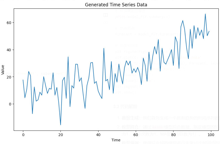
# 可视化原始数据
plt.figure(figsize=(10, 6))
plt.plot(t, series)
plt.title('Generated Time Series Data')
plt.xlabel('Time')
plt.ylabel('Value')
plt.show()

# 拟合ARIMA(1,1,1)模型，p=1, d=1, q=1
model = ARIMA(series, order=(1, 1, 1))
model_fit = model.fit()

# 打印模型的概况
print(model_fit.summary())

# 做出预测
forecast = model_fit.forecast(steps=10)

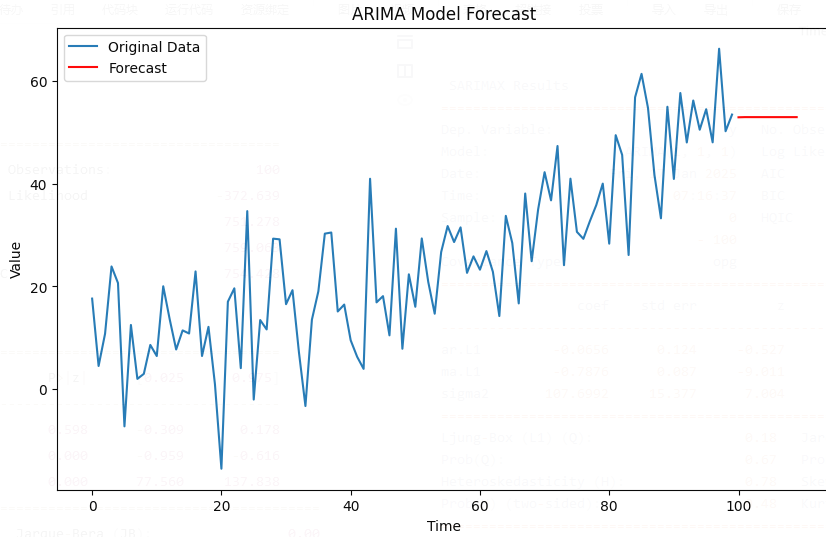
# 可视化结果
plt.figure(figsize=(10, 6))
plt.plot(t, series, label='Original Data')
plt.plot(t[-1] + np.arange(1, 11), forecast, label='Forecast', color='red')
plt.title('ARIMA Model Forecast')
plt.xlabel('Time')
plt.ylabel('Value')
plt.legend()
plt.show()

3.3 代码解释

1. 数据生成：我们首先生成一个具有趋势的时间序列数据，其中包含一定的噪声。
2. 模型拟合：通过ARIMA模型拟合数据，指定模型的阶数（这里是(1, 1, 1)，表示AR部分的阶数为1，差分次数为1，MA部分的阶数为1）。
3. 模型预测：使用拟合好的模型进行未来10个时间点的预测，并绘制预测结果。

3.4 输出结果

通过上面的代码，我们可以得到模型的拟合结果和未来数据点的预测，通常结果会包括系数的估计值、标准误差、AIC/BIC等评估指标。

 SARIMAX Results                                
==============================================================================
Dep. Variable:                      y   No. Observations:                  100
Model:                 ARIMA(1, 1, 1)   Log Likelihood                -372.639
Date:                Fri, 17 Jan 2025   AIC                            751.278
Time:                        07:16:37   BIC                            759.063
Sample:                             0   HQIC                           754.428
                                - 100                                         
Covariance Type:                  opg                                         
==============================================================================
                 coef    std err          z      P>|z|      [0.025      0.975]
------------------------------------------------------------------------------
ar.L1         -0.0656      0.124     -0.527      0.598      -0.309       0.178
ma.L1         -0.7876      0.087     -9.011      0.000      -0.959      -0.616
sigma2       107.6992     15.377      7.004      0.000      77.560     137.838
===================================================================================
Ljung-Box (L1) (Q):                   0.18   Jarque-Bera (JB):                 0.00
Prob(Q):                              0.67   Prob(JB):                         1.00
Heteroskedasticity (H):               0.78   Skew:                             0.01
Prob(H) (two-sided):                  0.48   Kurtosis:                         2.99
===================================================================================

Warnings:
[1] Covariance matrix calculated using the outer product of gradients (complex-step).

4. ARIMA模型的应用

ARIMA模型在经济、金融、气象等领域得到了广泛应用。以下是几个典型的应用场景：

4.1 股票市场预测

ARIMA模型广泛用于股票市场的价格预测。通过分析股票历史数据，ARIMA模型能够识别股票价格的趋势和周期性波动，进而预测未来的股价走势。

4.2 需求预测

在零售和供应链管理中，ARIMA模型常用于产品需求预测。通过对历史销售数据进行建模，企业可以预测未来的需求，帮助调整库存和生产计划。

4.3 经济数据分析

ARIMA模型也被广泛用于宏观经济数据的分析，例如GDP、失业率、通货膨胀等。通过对这些经济指标的时间序列进行分析，ARIMA模型能够揭示经济活动中的潜在趋势和波动。

5. 总结

ARIMA模型是一种强大的时间序列预测工具，适用于平稳和非平稳数据的建模。通过自回归（AR）、差分（I）和滑动平均（MA）三种方法，ARIMA能够帮助分析人员理解时间序列中的趋势和季节性，并进行有效的预测。在Python中，我们可以通过statsmodels库轻松实现ARIMA模型，并进行预测和模型评估。

ARIMA Model: A Powerful Tool for Time Series Analysis

The ARIMA (AutoRegressive Integrated Moving Average) model is a widely used model in time series analysis. By combining autoregression, differencing, and moving average techniques, it models and predicts time series data. This blog will give a detailed introduction to the ARIMA model’s basic principles, mathematical formulas, and Python implementation, as well as provide a numerical simulation example to showcase its application.

1. Basic Principles of the ARIMA Model

The core idea of the ARIMA model is to transform a non-stationary time series into a stationary series, and then model it using the three components: Autoregression (AR), Differencing (I), and Moving Average (MA). Specifically, the ARIMA model consists of three key components:

1.1 Autoregression (AR)

Autoregression (AR) refers to the relationship between the current value and its previous values. The AR process assumes that the current value is a linear combination of its past values. The order of autoregression (i.e., how many past values to use) is denoted by the parameter ( $p$ ).

The mathematical formula for AR is:
$$Y_t={\varphi }_1{Y}_{t-1}+{\varphi }_2{Y}_{t-2}+\cdots +{\varphi }_p{Y}_{t-p}+{ϵ}_t$$
where ( $Y_t$ ) is the observed value at time ( $t$ ), ( ${\varphi }_1,{\varphi }_2,\dots ,{\varphi }_p$ ) are the regression coefficients, and ( ${ϵ}_t$ ) is the error term.

1.2 Differencing (I)

Differencing (Integrated) is used to make a non-stationary time series stationary. By calculating the difference between consecutive time points, trends in the data can be removed. The order of differencing is denoted by ( $d$ ).

The differencing operation can be written as:
$$\Delta Y_t=Y_t-Y_{t-1}$$
Here, ( $\Delta Y_t$ ) represents the differenced time series.

1.3 Moving Average (MA)

Moving Average (MA) refers to modeling the current value as a linear combination of past error terms. The order of MA is denoted by ( $q$ ).

The mathematical formula for MA is:
$$Y_t=\mu +{ϵ}_t+{\theta }_1{ϵ}_{t-1}+{\theta }_2{ϵ}_{t-2}+\cdots +{\theta }_q{ϵ}_{t-q}$$
where ( ${ϵ}_t$ ) is the error term at time ( $t$ ), and ( ${\theta }_1,{\theta }_2,\dots ,{\theta }_q$ ) are the moving average coefficients.

1.4 ARIMA Model Formula

The overall mathematical formula of the ARIMA model can be written as:
$$Y_t=\mu +{\varphi }_1{Y}_{t-1}+\cdots +{\varphi }_p{Y}_{t-p}+{\theta }_1{ϵ}_{t-1}+\cdots +{\theta }_q{ϵ}_{t-q}+{ϵ}_t$$
where ( $\mu$ ) is the constant term, ( $\varphi$ ) and ( $\theta$ ) are the coefficients of the AR and MA components, and ( ${ϵ}_t$ ) is the error term.

2. ARIMA Model Parameter Selection

Choosing the right parameters for the ARIMA model depends on the characteristics of the data. Typically, the following steps are followed to determine the best parameters:

1. Stationarity Check: First, check whether the time series is stationary. If the series is non-stationary, differencing (I) is needed.
2. ACF and PACF Analysis: Analyze the Autocorrelation Function (ACF) and Partial Autocorrelation Function (PACF) plots to determine the order of AR and MA.
   • ACF plot is mainly used to determine the order of MA.
   • PACF plot is used to determine the order of AR.
3. Model Fitting and Evaluation: After selecting the parameters, fit the ARIMA model and evaluate it using criteria like AIC (Akaike Information Criterion) and BIC (Bayesian Information Criterion).

3. Python Code Implementation of ARIMA

Below is an example Python code that implements the ARIMA model using the statsmodels library. It includes data generation, ARIMA model fitting, and prediction.

3.1 Install Required Libraries

First, make sure to install the required libraries: statsmodels and matplotlib.

pip install statsmodels matplotlib

3.2 Code Implementation

import numpy as np
import pandas as pd
import matplotlib.pyplot as plt
from statsmodels.tsa.arima.model import ARIMA

# Generate synthetic time series data
np.random.seed(0)
n = 100
t = np.arange(n)
data = 0.5 * t + np.random.normal(0, 10, n)  # Generate time series data with trend

# Convert to pandas Series
series = pd.Series(data)

# Plot the original data
plt.figure(figsize=(10, 6))
plt.plot(t, series)
plt.title('Generated Time Series Data')
plt.xlabel('Time')
plt.ylabel('Value')
plt.show()

# Fit ARIMA(1,1,1) model, p=1, d=1, q=1
model = ARIMA(series, order=(1, 1, 1))
model_fit = model.fit()

# Print model summary
print(model_fit.summary())

# Make predictions
forecast = model_fit.forecast(steps=10)

# Plot the results
plt.figure(figsize=(10, 6))
plt.plot(t, series, label='Original Data')
plt.plot(t[-1] + np.arange(1, 11), forecast, label='Forecast', color='red')
plt.title('ARIMA Model Forecast')
plt.xlabel('Time')
plt.ylabel('Value')
plt.legend()
plt.show()

3.3 Code Explanation

1. Data Generation: First, we generate synthetic time series data with a trend, adding some noise.
2. Model Fitting: We fit the ARIMA model with the specified order ( $(1,1,1)$ ), meaning 1 autoregressive term, 1 differencing, and 1 moving average term.
3. Prediction: The forecast() method is used to predict the next 10 time points. The results are plotted alongside the original data for comparison.

3.4 Output

Running the code will give the summary of the ARIMA model’s fit and plot the original time series alongside the forecasted values. The model summary will include parameter estimates, standard errors, and evaluation criteria such as AIC and BIC.

4. Applications of the ARIMA Model

ARIMA is a powerful tool for time series forecasting and is applied in various fields such as economics, finance, and meteorology. Here are a few typical applications:

4.1 Stock Market Prediction

ARIMA is widely used for stock market price prediction. By analyzing historical stock data, ARIMA can identify trends and cyclical patterns, which helps in predicting future stock prices.

4.2 Demand Forecasting

In retail and supply chain management, ARIMA models are used for demand forecasting. By modeling past sales data, businesses can predict future demand, which helps in inventory management and production planning.

4.3 Economic Data Analysis

ARIMA is also extensively used for analyzing macroeconomic data such as GDP, unemployment rates, and inflation. By modeling these economic indicators, ARIMA can uncover underlying trends and fluctuations in economic activity.

5. Conclusion

The ARIMA model is a powerful tool for time series forecasting, suitable for both stationary and non-stationary data. By using autoregression (AR), differencing (I), and moving average (MA), ARIMA helps uncover trends and seasonality in time series data. In Python, the statsmodels library provides an easy-to-use implementation for fitting ARIMA models and making predictions.

后记

2025年1月17日15点16分于上海，在GPT4o大模型辅助下完成。