大数据课程笔记4：摘要结构，streaming algorithm

这是大数据课程第四节的笔记，笔者自己的理解使用斜体注明，正确性有待验证。

This is the note of lecture 4 in Big Data Algorithm class. The use of italics indicates the author’s own understanding, whose correctness needs to be verified.

---

1. Synopsis Structure

Most contents of the synopsis structure are collected from the lecture note in http://www.cohenwang.com/edith/bigdataclass2013 .

1.1. Definition

A small summary of a large data set that (approximately) captures some statistics/properties we are interested in.

Example: random samples, sketches/projections, histograms,…

1.2. Functionality

Some operations, such as insertion, deletion, query and merging databases, may be required.

1.3. Motivation/ Why?

Data can be too large to

1. Keep for long or even short term
2. Transmit across the network
3. Process queries over in reasonable time/computation

1.4. Limitation

The size of working cpu/memory can be limited compared with the size of data.

Only one or two passes of data in cpu are affordable.

1.5. Applications:

network traffic management

I/O Efficiency

Real Time Data

2. Frequent Elements: Misra Gries Algorithm

2.1. Purpose

In brief, the system reads the data in one pass and outputs the frequencies of the top-k most frequent elements.

2.2. Motivation/Application

zipf law: Typical frequency distributions are highly skewed: with few very frequent elements. Say top 10% of elements have 90% of total occurrences. We are interested in finding the heaviest elements.

According to the zipf law, the most frequent elements are significant to represent the data.

Some applications:

1. Networking: Find “elephant” flows
2. Search: Find the most frequent queries

2.3. A simple algorithm

Simply create a counter for each distinct element and count it in its following occurrence.

However, this algorithm requires about $n\log m$ bits, where $n$ is the number of distinct elements, and $m$ denotes the total number of elements. Sometimes, $n$ counters are too large and only $k$ counters are affordable.

2.4. Misra Gries Algorithm

2.4.1. Insert, Query

1. Place a counter on the first k distinct elements.
2. On the (k + 1)-st elements, reduce each counter by 1 and remove counters of value zero.
3. Report counter value on any query.

2.4.2. One simple example for Insertion and Query

The input stream is “abccbcbae” (simply chosen randomly), and the maximum counter number k is 2.

step number	current element	counter1’s element	counter1’s value	counter2’s element	counter2’s value
0	a	a	1	-	-
1	b	a	1	b	1
2	c	-	-	-	-
3	c	c	1	-	-
4	b	c	1	b	1
5	c	c	2	b	1
6	b	c	2	b	2
7	a	c	1	b	1
8	e	-	-	-	-

2.4.3. Analyze the output

As illustrated in the previous example, the output is obviously an underestimate. However the maximum error is limited. When zipf law / power law property of data holds, the error is acceptable.

$m$ is the total number of elements in the input, and $m'$ is the sum of the output. For example, $m$ is $9$ and $m'$ is $0$ in step $2$ and $4$ in step $6$ in the previous example. If $n\le k$, $m=m'$, since if there is no (k + 1)-st elements, there is no reduction or removement. If $n>k$, the difference between $m$ and $m'$ is caused by the reduction operations. And for each reduction operation, $k+1$ is reduced from the current output. Then there are at most $\frac{m-m'}{k+1}$ reduction operations. Moreover, for each counter, the number is reduced by at most $1$ for each reduction operation. Then the number is reduced by at most $\frac{m-m'}{k+1}$.

The error is proportional to the inverse of $k$. So the error is small when memory is large enough. Furthermore, when $k$ is fixed, it’s proportional to $m-m'$. Notice that $m$ is the total number of input elements, $m'$ is the estimate of the total number of the top $k$ most frequent elements. So the output is more accurate, if zipf law holds and $m$ is large enough. This conclusion also explains the poor estimate in the example.

2.4.4. Merge

The merge operation is similar to insertion, as following:

1. Merge the common element counter, keep distinct counters.
2. Remove small counters to keep k largest (by reducing counter then remove counters of value zero.

The estimate error is also at most $\frac{m-m'}{k+1}$. More details can be found in the lecture note in http://www.cohenwang.com/edith/bigdataclass2013 .

3. Stream Counting

3.1. Purpose

The system reads the data in one pass and output the total number of elements. It’s simply a counter.

3.2. A simple algorithm

One simple way is to keep one number as the counter, which increases by one for each element read.

The required space $O(\log N)$, where $N$ is the total number of input.

3.3. Morris’s idea

Instead of counting store $N$ in $\log N$ bits, it will store $\log N$ in $\log\log N$ bits. It may take advantage of the idea that when N is large, the exact number of $N$ is not important compared with the size of $N$. For example, when $N=100000000$, it doesn’t matter whether $N=100000010$ or $N=100000000$. However, that the left most $1$ is in the $9$th position is important.

It also uses the powerful tool: randomization, and guarantee that the expectation of the output is the same as the correct output, while saving space.

The algorithm is as follows:

1. Keep a counter $x$ of value “$\log n$”.
2. Increase the counter with probability $p = 2^{-x}$ .
3. On a query, return $2^x-1$.

3.4. One example

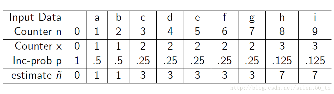
3.5. Analyze: the expected return value

The claim: Expected value after reading $n$ input data is $n$.

Proof: Using the inductive principle, the proof is simple.

1. Base case: $n=0$, $x=0$ ,$\hat n = 2^x-1=0 = n$. Base case approved.
2. Assume the claim is true for all $n\le k$, which means $EX[\hat n] = n$.
3. When $n=k+1$, we have

$$EX[\hat n] = EX(2^{x_n}-1)~~~~~~~~~~~~~~~~~~~~~~~~~~~~~~~~~~~~~~~~~~~~~~~~~~~~~~~~~~~~~~~~~~~~~~~~~~~~~~~~~~~~~~~~~~~~~~~~ ~~~~~~~~~~~~~~~~~~~~~~~~\\ = \sum_{\text{all }j\ge 1} P(x_{n-1} = j)EX(2^{x_n}|x_{n-1}=j)-1~~~~~~~~~~~~~~~~~~~~~~~~~~~~~~~~~~~~~~~~~~~~~~~~~~~~~~~~~~~~~ \\ = \sum_{\text{all }j\ge 1} P(x_{n-1} = j)[P(x_n=j+1|x_{n-1}=j)2^{j+1}+P(x_n=j|x_{n-1}=j)2^j]-1 \\ = \sum_{\text{all }j\ge 1} P(x_{n-1} = j)[2^{-j}2^{j+1}+(1-2^{-j})2^j]-1~~~~~~~~~~~~~~~~~~~~~~~~~~~~~~~~~~~~~~~~~~~~~~~~~~~~ \\ = \sum_{\text{all }j\ge 1} P(x_{n-1} = j)[2^j+1]-1 ~~~~~~~~~~~~~~~~~~~~~~~~~~~~~~~~~~~~~~~~~~~~~~~~~~~~~~~~~~~~~~~~~~~~~~~~~~~~~~~\\ = \sum_{\text{all }j\ge 1} P(x_{n-1} = j)[2^j-1]+1 ~~~~~~~~~~~~~~~~~~~~~~~~~~~~~~~~~~~~~~~~~~~~~~~~~~~~~~~~~~~~~~~~~~~~~~~~~~~~~~~\\ =EX(x_{n-1})+1~~~~~~~~~~~~~~~~~~~~~~~~~~~~~~~~~~~~~~~~~~~~~~~~~~~~~~~~~~~~~~~~~~~~~~~~~~~~~~~~~~~~~~~~~~~~~~~~~~~~~~~~\\ =k+1~~~~~~~~~~~~~~~~~~~~~~~~~~~~~~~~~~~~~~~~~~~~~~~~~~~~~~~~~~~~~~~~~~~~~~~~~~~~~~~~~~~~~~~~~~~~~~~~~~~~~~~~~~~~~~~~~~~~~~~$$

According to the principle of induction, the claim is true for all $n\ge 0$.

4. Count Distinct Items

4.1. Some definitions

Input sequence $A=\{a_1,a_2,\cdots,a_m\}$, where $m$ is the number of elements. $a_i \in N=\{1,2,\cdots,n\}$. Therefore, there are no more than $n$ distince elements in $A$.

Define $m_i=\{j:a_j=i\}$, which is a set containing the index of all elements whose value is equal to $i$.

Then $F_k = \sum_{i=1}^{n}m_i^k,k = 0,1,2,\cdots$.

1. $F_0$ is the number of distince elements in list, since $\emptyset^0=0, S^0=1\text{ iff. }S\neq \emptyset$。
2. $F_1$ is the length of sequnce, $m$.
3. $F_2$ is called Ginis index of homogeneity.
4. $F^*_\infty=\max_{1\le i\le n}m_i$

4.2. Purpose

The system reads the data in one pass and outputs $F_0$, which is the number of distinct items in the input sequence.

4.3. General Theorem

4.4. Improved Performance

The memory size is $O(\log n)$ bits.

The property of output: $P( Y/F_0< 1/c)+P(Y/F_0> c)\le 3/c$, where $c$ is a fixed constant bigger than $2$, $Y$ is the estimated output.

4.5. Algorithm

The basic idea is firstly using the finite field to hash elements to reduce size and make the item randomized, and then using the property of $F_0$ random elements to estimate the size.

4.5.1. Basic Knowledge: Finite Field and Probability

Here, we only introduce some basic idea and calculation of finite field and probability. More details are available on the Internet.

4.5.1.1. Finite Field

Two websites, which explain the idea of finite field in detail, are found: http://mathworld.wolfram.com/FiniteField.html, http://blog.csdn.net/luotuo44/article/details/41645597

4.5.1.2. Probability Inequalities

1. Markov Inequality

   $P[X\ge d]\le \frac{EX[X]}{d}$ for $X\ge 0$.

   since $EX[X] = \int xf(x)dx \ge \int_{x=d} xf(x)dx \ge d\int_{x=d} f(x)dx$, where $f(x)$ is PDF (probability density function) of $X$.

2. Chebyshev Inequality

   $P[|X-\mu|\ge k\delta]\le \frac 1{k^2}$,

   since $P[|X-\mu|\ge k\delta] = P[(X-\mu)^2\ge k^2\delta^2] \le \frac{EX[(x-\mu)^2]}{k^2\delta^2} = \delta^2/(k^2\delta^2) = 1/k^2$, where $\mu=EX[X]$, $\delta=\text{Var}[X]$, $k$ is a fixed constant.

4.5.2. The algorithm

1. Construct the finite field $F=GF(2^d)$, where $n < 2^d$.

2. hash the input element
   
   1. $a, b$ randomly chosen from $F$.
   2. $\forall a_i \in A$ (in the order of the input sequence), hash $a_i$ to $z_i = a \times a_i + b(\text{mod }F)$ represented by a $d$-vector in $F$.
3. Estimate $F_0$ using properties of $F_0$ random values
   
   1. De fine $r_i = r(z_i ) = \max\{i:2^i|z_i\}$, such that $r_i$ is right most $1$’s position. For example $r(1010000)=4$ and $r(1010010) = 1$. $r_i$ should be less than $d$ , which is roughly $\log n$.
   2. Define $R$ to be the largest $r_i$ over all elements of A, which means $R=\max(r_1,r_2,\cdots,r_m)$
4. Output $Y=2^R$.

4.5.3. Some analysis of the algorithm

The use of the finite field is to hash input elements $a_i$ into a fixed size output $z_i$, which is uniformly distributed among $0$ and $2^d-1$. The fixed size output guarantees that the system requires a fixed size of space. Moreover, the randomized property guaranteed that $R$ can represent $F_0$.

Now let’s focus on the property of the output $Y$. Firstly, we need derive the probability distribution of $r_i$ based on $F_0$ different randomized elements. Since the elements are randomized, $p(r_i\ge j) = 2^{-j}$ . ($r_i\ge j$ means the last $j$ bits of the $i$th elements are all zero. The probability for each bit to be zero is $1/2$ since the the elements are randomized.) Furthermore, we define a new variable $Z_r=\sum_{x\in F_0}I[r(ax+b)\ge r]$, which is the number of elements with $r(ax+b)$ greater than $r$. According to the definition, we have $Z_R\ge 1$ and $Z_{R+1}=0$, where $R=\max(r_1,r_2,\cdots,r_m)$. The distribution of $Z_r$ is simply a bernoulli distribution of $N=F_0$ and $p = p(r_i\ge r) = 2^{-r}$. Then $E(Z_r) = F_02^{-r}$ and $\text{Var}(Z_r) = F_02^{-r}(1-2^{-r}) < E(Z_r)$.

As discussed above, $Y$ is related to $R$ by $Y=2^R$, and $R$ is related to $Z$ by $Z_R\ge 1$ and $Z_{R+1}=0$. When furthermore should discuss the probability of $P(Z_r\ge 1)$ and $P(Z_r=0)$.

$P(Z_r\ge 1)\le \frac{EX(Z_r)}{1} = F_0/2^r​$

$P(Z_r=0)\le P(|Z_r-E(Z_r)|\ge E(Z_r)) \le \frac{1}{E(Z_r)^2/\text{Var}(Z_r)}\le \frac 1{E(Z_r)} = 2^r/F_0$

If $2^r>cF_0$, then $P(Z_r\ge 1)\le 1/c$. Then $P(F_0/Y<1/c)=P(2^R>cF_0\text{ and } Z_R\ge1\text{ and } Z_{R+1}=0)\le P(Z_R\ge 1|2^R>cF_0)\le 1/c$

If $c*2^r< F_0$, then $P(Z_r=0)\le 1/c$. Then

$$P(F_0/Y>c)=P(c*2^R<F_0\text{ and }Z_R\ge1\text{ and }Z_{R+1}=0) \\ \le P(Z_{R+1}=0|c*2^R<F_0)\le \frac 1{E(Z_{R+1})}=2^{R+1}/F_0\le 2/c$$