


Step 6: Machine Learning
Machine Learning In Python: Intermediate
>>Multiclass classification:
pandas.get_dummies() 对dataframe或Series中value值进行变换,尤其是在value有多个取值时,转换为多个二进制的结果,
需要进行dummy处理的依据:针对于value之间没有明显的关系,即使数值很接近,但是意义完全分离的情况,例如:70,71代表年份,就可以dummy
#读取数据,输出origin的类别
import pandas as pd
cars = pd.read_csv("auto.csv")
unique_regions=cars['origin'].unique()
print(unique_regions)

#对数值类型进行转换
dummy_cylinders = pd.get_dummies(cars["cylinders"], prefix="cyl")
cars = pd.concat([cars, dummy_cylinders], axis=1)
dummy_years = pd.get_dummies(cars["year"], prefix="year")
cars = pd.concat([cars, dummy_years], axis=1)
cars=cars.drop(['cylinders','year'],axis=1)
print(cars.head())

#划分训练集与测试集
shuffled_rows = np.random.permutation(cars.index)
shuffled_cars = cars.iloc[shuffled_rows]
highest_train_row = int(cars.shape[0] * .70)
train = shuffled_cars.iloc[0:highest_train_row]
test = shuffled_cars.iloc[highest_train_row:]

#将三分类问题转化为三个二分类问题,给出两种解决方法
>>
from sklearn.linear_model import LogisticRegression
unique_origins = cars["origin"].unique()
unique_origins.sort()
models = {}
for i in unique_origins:
    model=LogisticRegression()
    train_x=train.iloc[:,6:]
    train_y=train['origin']==i
    model.fit(train_x,train_y)
    models[i]=model
>>
from sklearn.linear_model import LogisticRegression
unique_origins = cars["origin"].unique()
unique_origins.sort()
models = {}
features = [c for c in train.columns if c.startswith("cyl") or c.startswith("year")]
for origin in unique_origins:
    model = LogisticRegression()
    X_train = train[features]
    y_train = train["origin"] == origin
    model.fit(X_train, y_train)
    models[origin] = model

#计算各个模型对应类的概率值构成Dataframe表
testing_probs = pd.DataFrame(columns=unique_origins)
for i in unique_origins:
    testing_probs[i]=models[i].predict_proba(test[features])[:,1]

#根据最大概率确定分类
predicted_origins=testing_probs.idxmax(axis=1)
>>Intermediate Linear Regression:
线性模型评价指标: Sum of Square Error (SSE), Regression Sum of Squares (RSS), and Total Sum of Squares (TSS)
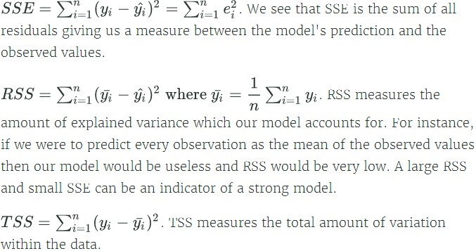
TSS=RSS+SSE
R-Squared: R^2=1-SSE/TSS=RSS/TSS 越大匹配效果越好
#披萨斜塔斜度随着时间的变化
import pandas
import matplotlib.pyplot as plt
pisa = pandas.DataFrame({"year": range(1975, 1988),
                         "lean": [2.9642, 2.9644, 2.9656, 2.9667, 2.9673, 2.9688, 2.9696,
                                  2.9698, 2.9713, 2.9717, 2.9725, 2.9742, 2.9757]})
print(pisa)
plt.scatter(x=pisa['year'],y=pisa['lean'])
plt.show()

import statsmodels.api as sm
y = pisa.lean # target
X = pisa.year  # features
X = sm.add_constant(X)  # add a column of 1's as the constant term
# OLS -- Ordinary Least Squares Fit
linear = sm.OLS(y, X)
# fit model
linearfit = linear.fit()
print(linearfit.summary())

# Our predicted values of y
yhat = linearfit.predict(X)
print(yhat)
residuals=yhat-y

# The variable residuals is in memory
plt.hist(residuals, bins=5)
import numpy as np
# sum the (predicted - observed) squared
SSE = np.sum((y.values-yhat)**2)
RSS=np.sum((y.mean()-yhat)**2)
TSS=SSE+RSS

#The models parameters
print("\n",linearfit.params)
delta = linearfit.params["year"] * 15

SSE = np.sum((y.values - yhat)**2)
# Compute variance in X
xvar = np.sum((pisa.year - pisa.year.mean())**2)
# Compute variance in b1
s2b1 = SSE / ((y.shape[0] - 2) * xvar)
R2=RSS/TSS

#画出T分布不同自由度曲线
from scipy.stats import t
# 100 values between -3 and 3
x = np.linspace(-3,3,100)
tdist3=t.pdf(x=x, df=3)
tdist30=t.pdf(x=x, df=30)
plt.plot(x,tdist3)
plt.plot(x,tdist30)
plt.show()

tstat = linearfit.params["year"] / np.sqrt(s2b1)
# At the 95% confidence interval for a two-sided t-test we must use a p-value of 0.975
pval = 0.975
# The degrees of freedom
df = pisa.shape[0] - 2
# The probability to test against
p = t.cdf(tstat, df=df)
beta1_test = p > pval
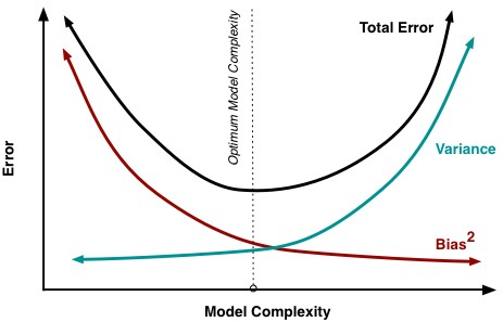
理想的模型复杂度的选择:
The best model was around 50% more accurate than the simplest model. On the other hand, the overall variance increased around 25% as we increased the model complexity.
# Our implementation for train_and_test, takes in a list of strings.
def train_and_test(cols):
    # Split into features & target.
    features = filtered_cars[cols]
    target = filtered_cars["mpg"]
    # Fit model.
    lr = LinearRegression()
    lr.fit(features, target)
    # Make predictions on training set.
    predictions = lr.predict(features)
    # Compute MSE and Variance.
    mse = mean_squared_error(filtered_cars["mpg"], predictions)
    variance = np.var(predictions)
    return(mse, variance)
one_mse, one_var = train_and_test(["cylinders"])
two_mse, two_var = train_and_test(['cylinders', 'displacement'])
three_mse, three_var = train_and_test(['cylinders', 'displacement', 'horsepower'])
four_mse, four_var = train_and_test(['cylinders', 'displacement', 'horsepower', 'weight'])
five_mse, five_var = train_and_test(['cylinders', 'displacement', 'horsepower', 'weight', 'acceleration'])
six_mse, six_var = train_and_test(['cylinders', 'displacement', 'horsepower', 'weight', 'acceleration', 'model year'])
seven_mse, seven_var = train_and_test(['cylinders', 'displacement', 'horsepower', 'weight', 'acceleration', 'model year', 'origin'])

#进行k折线交叉验证
from sklearn.cross_validation import KFold
from sklearn.metrics import mean_squared_error
import numpy as np
def train_and_cross_val(cols):
    features = filtered_cars[cols]
    target = filtered_cars["mpg"]
    variance_values = []
    mse_values = []
    # KFold instance.
    kf = KFold(n=len(filtered_cars), n_folds=10, shuffle=True, random_state=3)
    # Iterate through over each fold.
    for train_index, test_index in kf:
        # Training and test sets.
        X_train, X_test = features.iloc[train_index], features.iloc[test_index]
        y_train, y_test = target.iloc[train_index], target.iloc[test_index]
        # Fit the model and make predictions.
        lr = LinearRegression()
        lr.fit(X_train, y_train)
        predictions = lr.predict(X_test)
        # Calculate mse and variance values for this fold.
        mse = mean_squared_error(y_test, predictions)
        var = np.var(predictions)
        # Append to arrays to do calculate overall average mse and variance values.
        variance_values.append(var)
        mse_values.append(mse)
    # Compute average mse and variance values.
    avg_mse = np.mean(mse_values)
    avg_var = np.mean(variance_values)
    return(avg_mse, avg_var)
two_mse, two_var = train_and_cross_val(["cylinders", "displacement"])
three_mse, three_var = train_and_cross_val(["cylinders", "displacement", "horsepower"])
four_mse, four_var = train_and_cross_val(["cylinders", "displacement", "horsepower", "weight"])
five_mse, five_var = train_and_cross_val(["cylinders", "displacement", "horsepower", "weight", "acceleration"])
six_mse, six_var = train_and_cross_val(["cylinders", "displacement", "horsepower", "weight", "acceleration", "model year"])
seven_mse, seven_var = train_and_cross_val(["cylinders", "displacement", "horsepower", "weight", "acceleration","model year", "origin"])无监督的K-means方法与有监督的分类方法最大的区别是前者没有标签,后者是基于已知标签进行学习分类
import pandas as pd
import numpy as np
nba = pd.read_csv("nba_2013.csv")
point_guards=nba[nba['pos']=='PG']
point_guards['ppg'] = point_guards['pts'] / point_guards['g']
point_guards = point_guards[point_guards['tov'] != 0]
point_guards['atr']=point_guards['ast']/point_guards['tov']
#初始化,随机产生5个中心点
num_clusters = 5
# Use numpy's random function to generate a list, length: num_clusters, of indices
random_initial_points = np.random.choice(point_guards.index, size=num_clusters)
# Use the random indices to create the centroids
centroids = point_guards.loc[random_initial_points]
#5个中心点构成的字典
def centroids_to_dict(centroids):
    dictionary = dict()
    # iterating counter we use to generate a cluster_id
    counter = 0
    # iterate a pandas data frame row-wise using .iterrows()
    for index, row in centroids.iterrows():
        coordinates = [row['ppg'], row['atr']]
        dictionary[counter] = coordinates
        counter += 1
    return dictionary
centroids_dict = centroids_to_dict(centroids)

#计算欧几里得距离
import math
def calculate_distance(centroid, player_values):
    root_distance = 0
    for x in range(0, len(centroid)):
        difference = centroid[x] - player_values[x]
        squared_difference = difference**2
        root_distance += squared_difference
    euclid_distance = math.sqrt(root_distance)
    return euclid_distance

#给各个点进行标记
def assign_to_cluster(s):
    s_p=s.loc[['ppg','atr']]
    min_dis=None
    min_id=0
    for k,v in centroids_dict.items():
        k_dis=calculate_distance(v,s_p)
        if min_dis==None or min_dis>k_dis:
            min_dis=k_dis
            min_id=k
    return min_id
point_guards['cluster']=point_guards.apply(assign_to_cluster,axis=1)

#可视化
def visualize_clusters(df, num_clusters):
    colors = ['b', 'g', 'r', 'c', 'm', 'y', 'k']
    for n in range(num_clusters):
        clustered_df = df[df['cluster'] == n]
        plt.scatter(clustered_df['ppg'], clustered_df['atr'], c=colors[n-1])
        plt.xlabel('Points Per Game', fontsize=13)
        plt.ylabel('Assist Turnover Ratio', fontsize=13)
    plt.show()
visualize_clusters(point_guards, 5)

#继续迭代,更新各个簇的中心点,采用统计平均
def recalculate_centroids(df):
    new_centroids_dict = dict()
    # 0..1...2...3...4
    for cluster_id in range(0, num_clusters):
        # Finish the logic
        cluster_df=df[df['cluster']==cluster_id]
        new_centroids_dict[cluster_id]=(cluster_df['ppg'].mean(),cluster_df['atr'].mean())
    return new_centroids_dict
centroids_dict = recalculate_centroids(point_guards)

#继续可视化和迭代
point_guards['cluster'] = point_guards.apply(lambda row: assign_to_cluster(row), axis=1)
visualize_clusters(point_guards, num_clusters)
centroids_dict = recalculate_centroids(point_guards)
point_guards['cluster'] = point_guards.apply(lambda row: assign_to_cluster(row), axis=1)
visualize_clusters(point_guards, num_clusters)

#采用sklearn聚类的方式
from sklearn.cluster import KMeans
kmeans = KMeans(n_clusters=num_clusters)
kmeans.fit(point_guards[['ppg', 'atr']])
point_guards['cluster'] = kmeans.labels_
visualize_clusters(point_guards, num_clusters)import pandas
import matplotlib.pyplot as plt
pga = pandas.read_csv("pga.csv")
pga.distance = (pga.distance - pga.distance.mean()) / pga.distance.std()
pga.accuracy = (pga.accuracy - pga.accuracy.mean()) / pga.accuracy.std()
print(pga.head())
plt.scatter(pga.distance, pga.accuracy)
plt.xlabel('normalized distance')
plt.ylabel('normalized accuracy')
plt.show()
#线性模型
from sklearn.linear_model import LinearRegression
import numpy as np
model=LinearRegression()
model.fit(pga[['distance']],pga['accuracy'])
theta1=model.coef_
#损失函数
def cost(theta0, theta1, x, y):
# Initialize cost
J = 0
# The number of observations
m = len(x)
# Loop through each observation
for i in range(m):
# Compute the hypothesis
h = theta1 * x[i] + theta0
# Add to cost
J += (h - y[i])**2
# Average and normalize cost
J /= (2*m)
return J
#画出三维图
theta0s = np.linspace(-2,2,100)
theta1s = np.linspace(-2,2, 100)
COST = np.empty(shape=(100,100))
T0S, T1S = np.meshgrid(theta0s, theta1s)
for i in range(100):
for j in range(100):
COST[i,j] = cost(T0S[0,i], T1S[j,0], pga.distance, pga.accuracy)
fig2 = plt.figure()
ax = fig2.gca(projection='3d')
ax.plot_surface(X=T0S,Y=T1S,Z=COST)
plt.show()
#求斜率和截距的偏导数
def partial_cost_theta1(theta0, theta1, x, y):
# Hypothesis
h = theta0 + theta1*x
# Hypothesis minus observed times x
diff = (h - y) * x
# Average to compute partial derivative
partial = diff.sum() / (x.shape[0])
return partial
def partial_cost_theta0(theta0, theta1, x, y):
# Hypothesis
h = theta0 + theta1*x
# Difference between hypothesis and observation
diff = (h - y)
# Compute partial derivative
partial = diff.sum() / (x.shape[0])
return partial
#梯度下降算法
# x is our feature vector -- distance
# y is our target variable -- accuracy
# alpha is the learning rate
# theta0 is the intial theta0
# theta1 is the intial theta1
def gradient_descent(x, y, alpha=0.1, theta0=0, theta1=0):
max_epochs = 1000 # Maximum number of iterations
counter = 0 # Intialize a counter
c = cost(theta1, theta0, pga.distance, pga.accuracy) ## Initial cost
costs = [c] # Lets store each update
# Set a convergence threshold to find where the cost function in minimized
# When the difference between the previous cost and current cost
# is less than this value we will say the parameters converged
convergence_thres = 0.000001
cprev = c + 10
theta0s = [theta0]
theta1s = [theta1]
# When the costs converge or we hit a large number of iterations will we stop updating
while (np.abs(cprev - c) > convergence_thres) and (counter < max_epochs):
cprev = c
# Alpha times the partial deriviative is our updated
update0 = alpha * partial_cost_theta0(theta0, theta1, x, y)
update1 = alpha * partial_cost_theta1(theta0, theta1, x, y)
# Update theta0 and theta1 at the same time
# We want to compute the slopes at the same set of hypothesised parameters
# so we update after finding the partial derivatives
theta0 -= update0
theta1 -= update1
# Store thetas
theta0s.append(theta0)
theta1s.append(theta1)
# Compute the new cost
c = cost(theta0, theta1, pga.distance, pga.accuracy)
# Store updates
costs.append(c)
counter += 1 # Count
return {'theta0': theta0, 'theta1': theta1, "costs": costs}
print("Theta1 =", gradient_descent(pga.distance, pga.accuracy)['theta1'])
descend = gradient_descent(pga.distance, pga.accuracy, alpha=.01)
plt.scatter(range(len(descend["costs"])), descend["costs"])
plt.show()注意矩阵相乘维度的问题,尤其是向量(0维)与矩阵(n*1维)是不一样的
x0 =[ 1. ,  7.4,  2.8,  6.1,  1.9]
# Initialize thetas randomly
theta_init = np.random.normal(0,0.01,size=(5,1))    #shape(5,1)
def sigmoid_activation(x,theta):
    v=np.dot([x],theta)				#(1,5)*(5,1)
    v1=1+np.exp(-v)
    return 1/v1[0]				#(1,1)[0]
def sigmoid_activation(x, theta):
    x = np.asarray(x)                           #shape(5,)
    theta = np.asarray(theta)			#shape(5,1)
    return 1 / (1 + np.exp(-np.dot(theta.T, x)))#(1,5)*(5,) 得到(1,)

a1=sigmoid_activation(x0,theta_init)
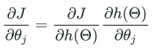
计算负梯度:

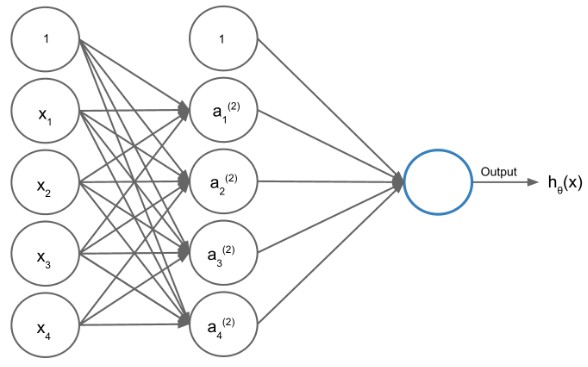
三层网络:
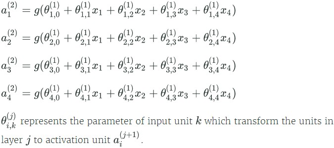

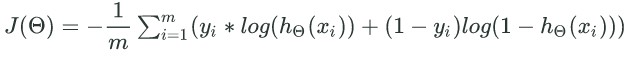
多层神经网络的损失函数:

#计算h(x)
iris["ones"] = np.ones(iris.shape[0])
X = iris[['ones', 'sepal_length', 'sepal_width', 'petal_length', 'petal_width']].values
y = (iris.species == 'Iris-versicolor').values.astype(int)
x0 = X[0]
theta_init = np.random.normal(0,0.01,size=(5,1))
def sigmoid_activation(x, theta):
    x = np.asarray(x)
    theta = np.asarray(theta)
    return 1 / (1 + np.exp(-np.dot(theta.T, x)))
a1 = sigmoid_activation(x0, theta_init)

#计算损失函数J
x0 = X[0]
y0 = y[0]
# Initialize parameters, we have 5 units and just 1 layer
theta_init = np.random.normal(0,0.01,size=(5,1))
def singlecost(X, y, theta):
    h = sigmoid_activation(X.T, theta)
    cost = -np.mean(y * np.log(h) + (1-y) * np.log(1-h))
    return cost
first_cost = singlecost(x0, y0, theta_init)

#计算梯度
theta_init = np.random.normal(0,0.01,size=(5,1))
grads = np.zeros(theta_init.shape)
n = X.shape[0]
for j, obs in enumerate(X):
    h = sigmoid_activation(obs, theta_init)
    delta = (y[j]-h) * h * (1-h) * obs
    grads += delta[:,np.newaxis]/X.shape[0]

#二层网络
theta_init = np.random.normal(0,0.01,size=(5,1))
# set a learning rate
learning_rate = 0.1
# maximum number of iterations for gradient descent
maxepochs = 10000
# costs convergence threshold, ie. (prevcost - cost) > convergence_thres
convergence_thres = 0.0001
def learn(X, y, theta, learning_rate, maxepochs, convergence_thres):
    costs = []
    cost = singlecost(X, y, theta)  # compute initial cost
    costprev = cost + convergence_thres + 0.01  # set an inital costprev to past while loop
    counter = 0  # add a counter
    # Loop through until convergence
    for counter in range(maxepochs):
        grads = np.zeros(theta.shape)
        for j, obs in enumerate(X):
            h = sigmoid_activation(obs, theta)   # Compute activation
            delta = (y[j]-h) * h * (1-h) * obs   # Get delta
            grads += delta[:,np.newaxis]/X.shape[0]  # accumulate
        # update parameters
        theta += grads * learning_rate
        counter += 1  # count
        costprev = cost  # store prev cost
        cost = singlecost(X, y, theta) # compute new cost
        costs.append(cost)
        if np.abs(costprev-cost) < convergence_thres:
            break
    plt.plot(costs)
    plt.title("Convergence of the Cost Function")
    plt.ylabel("J($\Theta$)")
    plt.xlabel("Iteration")
    plt.show()
    return theta
theta = learn(X, y, theta_init, learning_rate, maxepochs, convergence_thres)

#三层神经网络
theta0_init = np.random.normal(0,0.01,size=(5,4))
theta1_init = np.random.normal(0,0.01,size=(5,1))
def feedforward(X, theta0, theta1):
    a1 = sigmoid_activation(X.T, theta0).T
    a1 = np.column_stack([np.ones(a1.shape[0]), a1])
    out = sigmoid_activation(a1.T, theta1)
    return out
h = feedforward(X, theta0_init, theta1_init)

#计算多层网络损失函数
def multiplecost(x,y,theta0,theta1):
    h=feedforward(x,theta0,theta1)
    return -np.mean(y*np.log(h)+(1-y)*np.log(1-h))
c=multiplecost(X,y,theta0_init,theta1_init)
# Use a class for this model, it's good practice and condenses the code
class NNet3:
    def __init__(self, learning_rate=0.5, maxepochs=1e4, convergence_thres=1e-5, hidden_layer=4):
        self.learning_rate = learning_rate
        self.maxepochs = int(maxepochs)
        self.convergence_thres = 1e-5
        self.hidden_layer = int(hidden_layer)
    def _multiplecost(self, X, y):
        # feed through network
        l1, l2 = self._feedforward(X)
        # compute error
        inner = y * np.log(l2) + (1-y) * np.log(1-l2)
        # negative of average error
        return -np.mean(inner)
    def _feedforward(self, X):
        # feedforward to the first layer
        l1 = sigmoid_activation(X.T, self.theta0).T
        # add a column of ones for bias term
        l1 = np.column_stack([np.ones(l1.shape[0]), l1])
        # activation units are then inputted to the output layer
        l2 = sigmoid_activation(l1.T, self.theta1)
        return l1, l2
    def predict(self, X):
        _, y = self._feedforward(X)
        return y
    def learn(self, X, y):
        nobs, ncols = X.shape
        self.theta0 = np.random.normal(0,0.01,size=(ncols,self.hidden_layer))
        self.theta1 = np.random.normal(0,0.01,size=(self.hidden_layer+1,1))
        self.costs = []
        cost = self._multiplecost(X, y)
        self.costs.append(cost)
        costprev = cost + self.convergence_thres+1  # set an inital costprev to past while loop
        counter = 0  # intialize a counter
        # Loop through until convergence
        for counter in range(self.maxepochs):
            # feedforward through network
            l1, l2 = self._feedforward(X)
            # Start Backpropagation
            # Compute gradients
            l2_delta = (y-l2) * l2 * (1-l2)
            l1_delta = l2_delta.T.dot(self.theta1.T) * l1 * (1-l1)
            # Update parameters by averaging gradients and multiplying by the learning rate
            self.theta1 += l1.T.dot(l2_delta.T) / nobs * self.learning_rate
            self.theta0 += X.T.dot(l1_delta)[:,1:] / nobs * self.learning_rate
            # Store costs and check for convergence
            counter += 1  # Count
            costprev = cost  # Store prev cost
            cost = self._multiplecost(X, y)  # get next cost
            self.costs.append(cost)
            if np.abs(costprev-cost) < self.convergence_thres and counter > 500:
                break
# Set a learning rate
learning_rate = 0.5
# Maximum number of iterations for gradient descent
maxepochs = 10000
# Costs convergence threshold, ie. (prevcost - cost) > convergence_thres
convergence_thres = 0.00001
# Number of hidden units
hidden_units = 4
# Initialize model
model = NNet3(learning_rate=learning_rate, maxepochs=maxepochs,
              convergence_thres=convergence_thres, hidden_layer=hidden_units)
# Train model
model.learn(X, y)
# Plot costs
plt.plot(model.costs)
plt.title("Convergence of the Cost Function")
plt.ylabel("J($\Theta$)")
plt.xlabel("Iteration")
plt.show()

#划分训练集 测试集
X_train,y_train=X[:70,:],y[:70]
X_test,y_test=X[-30:,:],y[-30:]

#训练与预测
from sklearn.metrics import roc_auc_score
# Set a learning rate
learning_rate = 0.5
# Maximum number of iterations for gradient descent
maxepochs = 10000
# Costs convergence threshold, ie. (prevcost - cost) > convergence_thres
convergence_thres = 0.00001
# Number of hidden units
hidden_units = 4
# Initialize model
model = NNet3(learning_rate=learning_rate, maxepochs=maxepochs,
              convergence_thres=convergence_thres, hidden_layer=hidden_units)
model.learn(X_train, y_train)
yhat = model.predict(X_test)[0]
auc = roc_auc_score(y_test, yhat)数据集: here
对股票进行预测,主要介绍了提取一些新的特征,但是要注意时间顺序,不能让现在或未来的信息泄露来影响模型评估。


 1365
1365

 被折叠的 条评论
为什么被折叠?
被折叠的 条评论
为什么被折叠?
 到【灌水乐园】发言


