集成经验模态(EEMD)原理详解与python实现

希尔伯特黄变换(Hilbert-Huang transform,HHT)被认为是近年来以傅里叶变换为基础的线性和稳态谱分析的一个重大突破。而经验模态分解算法是希尔伯特黄变换的核心部分，该算法能把复杂的信号序列分解为若干个本征模态函数之和，由于经验模态分解算法在非线性、非平稳性信号分析上的优势，最近被广泛应用于故障诊断、时间序列降噪等任务中。

1 经验模态分解(EMD)

经验模态分解（Empirical mode decomposition,EMD）由Huang et al(1998)${}^{[1]}$提出，是一种数据自适应多分辨率技术，用于将信号分解为物理上有意义的分量(component)。EMD可以用于分析非线性和非平稳信号，方法是将原始信号递归式分解成具有不同分辨率的分量。分量又被称为本征模态函数(Intrinsic Mode Functions,IMFs)。与傅里叶变换、小波变换需要预先设定变换基函数不同，经验模态分解不使用固定函数或滤波器。
根据经验模态分解的特点，该方法用于时间序列的分解降噪有两大优势：

1. 适应非线性和非平稳过程；
2. 自适应性，无需选择预定义的变换基函数；

1.1 本征模态函数(IMF)

本征模态函数是一个单分量函数(monocomponent function)或具有一个瞬时频率的振荡模式(an oscillatory mode)，该分量需要满足两个条件：

1. 在整个分量的时间序列中，极值的数目和过零点的数目必须相等或相差1;
2. 在分量时间序列的任何点，由局部最大值（上包络线）和局部最小值（下包络线）定义的包络范围的平均值等于零；

1.2 sifting算法

用于经验模态分解提取本征模态函数的方法为sifting算法，这是一种迭代方法，算法步骤如下：

step1: 识别观测信号时间序列的极值点$x(t)$，包括局部极大值和极小值；
step2: 使用三次样条曲线插值法对局部极值点进行插值，以获得上下包络线$U(t)$和$L(t)$;
step3: 计算上下包络线的局部均值线，即$m(t)=\frac{1}{2}(U(t)+L(t))$;
step4: 当前信号时间序列减去局部均值，作为新的信号时间序列$h_1(t)$，$h_1(t)=x(t)-m(t)$；

重复步骤1-4，直到获得的本征模态函数满足两个条件，则迭代结束。在这一迭代过程中，可求得多个本征模态函数。最后一步的本征模态函数为残差分量。

用于停止sifting过程的一个常用标准是：在算法提取了$M-1$个本征模态函数后，得到的残差$r_M(Z)$也为本征模态函数或单调函数(monotonic function)。
从sifting算法原理可看出，理解经验模态分解的另一种视角是将信号视为叠加在较慢信号上的快速振荡。在提取快速振荡之后，EMD算法将剩余的较慢分量视为新信号，并再次将其视为叠加在较慢分量上的快速振荡。算法继续，直到达到某个退出标准。

1.3 原始序列重构

sifting算法求得本征模态函数后，可以通过叠加本征模态函数来重构原始信号时间序列$X(t)$：
$$X(t)=\sum _{m=1}^{M-1}IM{F}_m(t)+r_M(t)$$
式中m为sifting算法迭代次数，t为时间点。

---

2 集成经验模态分解(EEMD)

EMD算法存在的一个问题是模态混叠(mode mixing effect/modal aliasing)，模态混叠问题是指1）具有不同时间尺度的振荡(oscillations)被分在一个本征模态函数中； 2）具有相同时间尺度的振动被筛选成不同的本征模态函数。
为解决此问题，Wu and Huang(2009)${}^{[2]}$提出一种噪声辅助的EMD算法，即集成经验模态分解(Ensemble empirical mode decomposition, EEMD)。
集成经验模态分解具有比标准经验模态分解更强的尺度分离能力，该方法在几次迭代试验中向信号中添加不同序列的白噪声。由于在每次试验中增加的噪声不同，各次试验所得的本征模态函数与其他试验的相应本征模态函数之间不表现出任何相关性。如果试验次数足够，则可以通过对不同试验获得的本征模态函数进行平均集成来消除添加的噪声。

2.1 EEMD算法步骤

集成经验模态分解算法步骤如下：

step i: 在n次试验中,通过添加白噪声时间序列到原有信号时间序列构建新的时间序列，$Y_n(t)=X(t)+u_n(t)$，for n=1,…,N，N为集成试验的次数；
step ii: 基于EMD算法，被噪声污染的时间序列$Y_n(t)$可分解为一系列本征模态函数和残差的加和，即$Y_n(t)={\sum }_{m=1}^{M-1}IM{F}_m^{(n)}(t)+r_M^{(n)}(t)$；式中m为sifting算法迭代次数，n为集成次数。
step iii：步骤1和2重复迭代N次，每次迭代试验中，不同的白噪声时间序列$u(t)$被加入原有信号时间序列；
step iv: 通过平均集成N次试验求得的本征模态函数，获得最终的本征模态函数：$IM{F}_m^{ave}(t)=\frac{1}{N}{\sum }_{n=1}^{N}IM{F}_m^{(n)}(t)$

集成经验模态分解的关键参数

从EEMD算法的步骤中可看出，算法分解的效果取决于集成次数N和添加的白噪声的幅度A，N与A取值应满足如下关系：
$$\epsilon =\frac{A}{\sqrt{N}}$$
式中$\epsilon$为误差的最终标准差，由原始信号时间序列与EEMD算法求得的本征模态函数的总和之间的差值计算得到。
因此，可通过设置期望的误差的标准差的值$\epsilon$和集成次数$N$，来获得噪声振幅的取值$A$。

---

3 代码实现

3.1 参数详解

调用emd包的sift函数实现经验模态分解,输入的信号为1维时间序列：

# emd.sift.sift(X, sift_thresh=1e-08, max_imfs=None, verbose=None, imf_opts=None, envelope_opts=None, extrema_opts=None)
	# X: 1D input array containing the time-series data to be decomposed
	# sift_thresh: The threshold at which the overall sifting process will stop. (Default value = 1e-8)
	# max_imfs: The maximum number of IMFs to compute. 
	# imf_opts： Optional dictionary of keyword options to be passed to emd.get_next_imf
imf_opts = {'env_step_size': 1/3, 'stop_method': 'rilling'}# 指定可选参数
imf = emd.sift.sift(x, max_imfs=4, imf_opts=imf_opts)

调用ensemble_sift函数实现集成经验模态分解：

# emd.sift.ensemble_sift(X, nensembles=4, ensemble_noise=0.2, noise_mode='single', nprocesses=1, sift_thresh=1e-08, max_imfs=None, verbose=None, imf_opts=None, envelope_opts=None, extrema_opts=None)
	# nensembles： 集成次数N
	# ensemble_noise: 加入每次集成过程中的白噪声的标准差
imf = emd.sift.ensemble_sift(burst+n, max_imfs=5, nensembles=2, nprocesses=6, ensemble_noise=1, imf_opts=imf_opts)
emd.plotting.plot_imfs(imf)

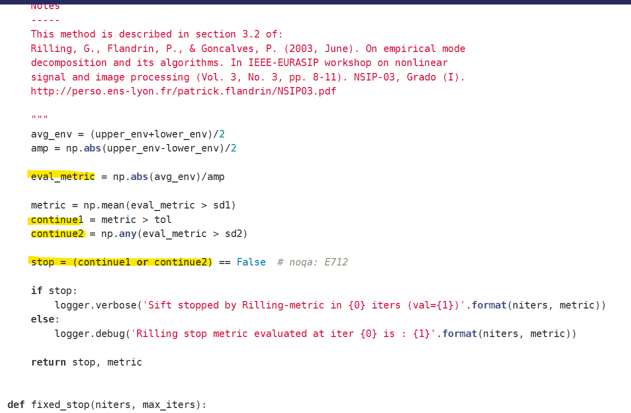
emd的高阶API中没有求残差分量的函数，从停止sift算法的源码来看，应该是sift算法达到停止标准时的最后一个IMF分量视为残差。

---

3.2 代码模版

使用经验模态分解算法对时间序列降噪：

def emd_model(ts):
    """
    parameter free model
    :param ts: 1d array shape:[样本数,]
    :return: imf ndarray shape:[样本数，模态分量数目]
    """
    imf_opts = {'sd_thresh': 0.05}  # 设置sift算法停止的默认阈值
    imf = emd.sift.sift(ts, imf_opts=imf_opts)
    emd.plotting.plot_imfs(imf)
    return imf

使用集成经验模态分解算法对时间序列降噪：

def eemd_model(ts,nensembles=2,ensemble_noise=1):
    """
    EEMD 模型
    :param ts: 1d array [sample,]
    :param nensembles: 集成次数
    :param ensemble_noise: 白噪声序列的标准差
    :return:
    """
    imf_opts = {'sd_thresh': 0.05} # 设置sift算法停止的默认阈值
    imf = emd.sift.ensemble_sift(ts, max_imfs=5, nensembles=nensembles, nprocesses=6, ensemble_noise=ensemble_noise, imf_opts=imf_opts)
    emd.plotting.plot_imfs(imf) # 绘制各本征模态分量的序列图
    return imf

分解后原序列、重构序列、残差分量可视化比较：

def emd_vis(imf):
    """
    see the residual , imf and orginal time series
    :param imf: 本征模态分量，[n_samples,n components]
    :return:
    """
    imfs,residual=imf[:,:-1],imf[:,-1]
    sum_imf=np.sum(imf[:,:-1],axis=1)
    plt.figure(figsize=(20, 10))
    plt.subplot(311)
    plt.plot(ts[:288 * 5], label='orginal series', color='blue')
    plt.plot(sum_imf, label="summed imf", color='green')
    plt.legend(loc='best')
    # plt.ylabel("orginal series")

    plt.subplot(312)
    plt.plot(residual)
    plt.ylabel("residual ")
    return

---

3.3 emd常用API函数

常用的底层函数API包括：

# 计算当前时间序列的下一个本征模态函数：
emd.sift.get_next_imf(X[, env_step_size, ...])
# Compute the next IMF from a data set. 
# 计算信号序列的上下包络线：
emd.sift.interp_envelope(X[, mode, ...]
# Interpolate the amplitude envelope of a signal.
# 求信号序列的极值点：
emd.sift.get_padded_extrema(X[, pad_width, ...])
# Identify and pad the extrema in a signal.
# 判断信号序列是否为本征模态函数，即满足两个条件：
emd.imftools.is_imf(imf[, avg_tol, ...])
 # Determine whether a signal is a 'true IMF'
# 求希尔伯特黄变换：
emd.spectra.hilberthuang(IF, IA[, edges, ...])
# Compute a Hilbert-Huang transform (HHT).
# 绘制sift获得的本征模态序列：
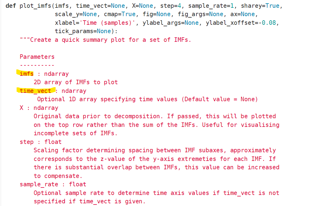
emd.plotting.plot_imfs(imf) # imf 2d arrary [samples,n_imfs]

其中，plot_imfs在emd的文档中没有参数解释，从源码中可看到该函数可通过time_vect参数定义绘图时的时间点坐标。

3.4 example demo

emd：

sample_rate = 512
seconds = 2
time_vect = np.linspace(0, seconds, seconds*sample_rate)
# Create an amplitude modulated burst
am = -np.cos(2*np.pi*1*time_vect) * 2
am[am < 0] = 0
burst = am*np.sin(2*np.pi*42*time_vect)
# Create some noise with increasing amplitude
am = np.linspace(0, 1, sample_rate*seconds)**2 + .1
np.random.seed(42)
n = am * np.random.randn(sample_rate*seconds,)
# Signal is burst + noise
x = burst + n
imf_opts = {'sd_thresh': 0.05}
imf = emd.sift.sift(burst+n, imf_opts=imf_opts)
emd.plotting.plot_imfs(imf)

---

eemd:

imf = np.zeros((x.shape[0], 5))
# Standard sift
imf[:, 0] = emd.sift.get_next_imf(x, **imf_opts)[0][:, 0]
# Additive noise sifts
imf = np.zeros((x.shape[0], 5))
# Additive noise sifts
noise_variance = 1
for ii in range(4):
    imf[:, ii+1] = emd.sift.get_next_imf(x + np.random.randn(x.shape[0],)*noise_variance, **imf_opts)[0][:, 0]

plt.figure()
plt.subplot(211)
plt.plot(imf[:, 0])
plt.subplot(212)
plt.plot(imf[:, 1:].mean(axis=1))

imf = emd.sift.ensemble_sift(burst+n, max_imfs=5, nensembles=2, nprocesses=6, ensemble_noise=1, imf_opts=imf_opts)
emd.plotting.plot_imfs(imf)

经验模态分解效果：

集成经验模态分解效果：

可以看到集成经验模态分解的效果要略优于经验模态分解，特别是最后两个分量的区分度更高。

---

参考资料

[1] Huang NE, Shen Z, Long SR, Wu MC, Shih EH, Zheng Q, Tung CC, Liu HH.The empirical mode decomposition method and the Hilbert spectrum for non-stationary time series analysis. Proc. Roy. Soc. London, vol. 454A, pp 903-995, 1998.
[2] Wu ZH, Huang NE. Ensemble empirical mode decomposition: a noise-assisted data analysis Method. AADA: Advances in Adaptive Data Analysis, vol. 1, pp.1-4. 2009.
[3] 蔡艳平,李艾华,徐斌,许平,何艳萍.集成经验模态分解中加入白噪声的自适应准则[J].振动.测试与诊断,2011,31(06):709-714+811.DOI:10.16450/j.cnki.issn.1004-6801.2011.06.003.
[4] Gaci S. A new ensemble empirical mode decomposition (EEMD) denoising method for seismic signals[J]. Energy Procedia, 2016, 97: 84-91.
[5] Zhang S, Zhou L, Chen X, et al. Network‐wide traffic speed forecasting: 3D convolutional neural network with ensemble empirical mode decomposition[J]. Computer‐Aided Civil and Infrastructure Engineering, 2020, 35(10): 1132-1147.
[6] emd package documentation
[7] https://gitlab.com/emd-dev/emd/-/blob/master/emd/plotting.py
[8] https://gitlab.com/emd-dev/emd/-/blob/master/emd/sift.py